The Kelly Criterion for Strategies: How to Size Positions and Allocate Capital

A strategy with positive expected value can still blow up your account if you get the bet size wrong. We walk through the Kelly criterion from deriving the formula to a portfolio of strategies: why full Kelly is dangerous, how fractional Kelly captures 75% of the growth at half the volatility, and what sizing recipe you should actually apply in algorithmic trading. Midway through the article there is an interactive calculator that shows how the Kelly fraction moves return and risk.
The question every strategy is obliged to answer
You have a strategy with a positive edge: over the long run it makes money. One detail remains — what fraction of capital to put into a single trade or to allocate to a single strategy.
This is not a secondary question but the central one. Positive expected value does not save you from ruin: bet too much, and a losing streak drives your account into a zone from which there is no statistical recovery (see The asymmetry of losses and gains). Bet too little, and you leave most of the potential growth on the table.
The Kelly criterion gives a precise answer: it is the fraction of capital that maximizes the long-term growth rate — the geometric one, not the arithmetic one. It is geometric growth that determines where your account ends up after a thousand trades, because returns multiply rather than add (see The multiplicative nature of returns).
Where the formula comes from: maximizing the logarithm of capital
The key idea of Kelly (1956) and later Thorp: what you should optimize is not the expected profit of a single trade but the expected logarithm of your final capital. The logarithm does not appear by accident — it is the only function whose maximization makes capital grow at the maximum geometric rate.
The binary case: a bet with two outcomes
Suppose that with probability the bet returns a net payout of per unit (the odds), and with probability we lose the stake itself. We bet a fraction of our capital. After one trade the capital is multiplied by on a win and by on a loss.
Expected log growth:
Take the derivative with respect to and set it to zero:
The solution is the Kelly formula:
In words: the optimal fraction equals your edge divided by the odds. No edge () — no bet.
Example
A strategy wins 55% of trades with a 1:1 payout ratio ():
Full Kelly tells you to risk 10% of capital per trade. Remember this number — below we will see why almost no one should bet exactly that much.
The continuous case: returns instead of bets
In trading a trade rarely looks like a bet with two outcomes — there is a distribution of returns. For returns with mean and variance per period, the expected log growth at leverage (fraction) is approximately:
The maximum is reached at:
This is the famous continuous form of Kelly (also known as the Merton fraction). And the growth rate at the optimum is tied to the Sharpe ratio in a remarkably elegant way:
A conclusion worth pinning to the wall: the maximum geometric growth rate of a portfolio equals half the square of its Sharpe. Double the Sharpe, and you quadruple the growth rate of capital.
Why full Kelly is too much
The formula gives the mathematical optimum for growth. But this optimum has a price the formula stays silent about: monstrous path volatility and drawdowns that break any real account and any real person.
The geometry of deviating from the optimum
Substitute the fraction (where is the Kelly multiplier: is full Kelly, is half Kelly) into the growth formula. Relative to the maximum we get:
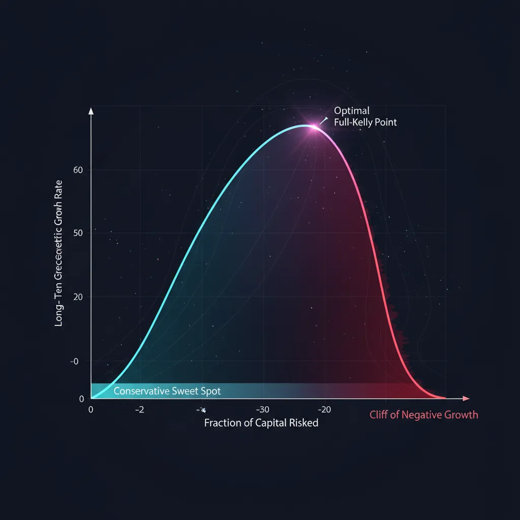
This parabola tells the entire story of risk management in a single line:
| Multiplier | Share of growth | Volatility | Comment |
|---|---|---|---|
| 0.25 (quarter) | 43.8% | 25% | almost half the growth at a quarter of the risk |
| 0.50 (half) | 75.0% | 50% | the practitioners' sweet spot |
| 1.00 (full) | 100.0% | 100% | maximum growth, wild volatility |
| 1.50 | 75.0% | 150% | the same growth as half, but triple the risk |
| 2.00 (double) | 0.0% | 200% | no growth, maximum risk |
| > 2.00 | negative | — | ruin despite a positive edge |
Three takeaways:
- half Kelly captures 75% of the growth at half the volatility. On a risk/return basis this is far better than full Kelly.
- The parabola is symmetric about . Betting Kelly gives the same growth as , but is three times more volatile. Overshooting is punished more harshly than undershooting.
- At Kelly growth goes to zero, and beyond that it turns negative. Sizing that is too aggressive kills capital even for a winning strategy.
Full Kelly drawdowns: the formula that sobers you up

For the continuous model, the probability that capital will ever fall to a fraction of its starting value equals:
Plug in the Kelly levels — and you get a table after which full Kelly stops looking attractive:
| Multiplier | P(ever −50%) | P(ever −75%) |
|---|---|---|
| 1.00 (full) | 50% | 75% |
| 0.50 (half) | 12.5% | 1.6% |
| 0.25 (quarter) | 0.78% | 0.006% |
| 2.00 (double) | 100% | 100% |
Under full Kelly the probability of ever seeing a 50% drawdown equals 50%. This is not a tail scenario — it is a coin flip. half Kelly knocks it down to 12.5%, quarter Kelly to a fraction of a percent. And that is in an idealized Gaussian model; real fat tails make actual drawdowns even deeper.
The calculator: move the Kelly fraction — watch return and risk
Move the sliders. The top two set the strategy's edge (win probability and payout ratio), the bottom one sets the Kelly multiplier . Watch how the growth rate of capital and the probability of a deep drawdown change at the same time. Pay attention to the article's main plot: as you move from half to full Kelly, growth rises a little, while drawdown risk rises several-fold.
Play with the Kelly fraction slider around the values 0.5 and 1.0: the growth versus maximum rises from 75% to 100%, but the risk of a 50% drawdown jumps from 13% to 50%. This is exactly why professionals live in the left half of the parabola.
Fractional Kelly as the industry standard
Serious managers almost never bet full Kelly. The typical range is from to Kelly. Beyond drawdowns there are four fundamental reasons to cut the fraction.
1. Parameter estimation error. The formula assumes you know the true , , , . In reality you estimate them from a finite sample. And the growth function is asymmetric: overestimating the edge pushes you past the optimum, where growth falls faster than it rises under the same underestimation. If the true Kelly equals and you estimated it with error, it is safer to systematically bet less. Rule of thumb: when the estimate is uncertain, halve the fraction.
2. Non-stationarity. A strategy's edge is not a constant — market regimes change, the edge decays, competitors copy the idea. The Kelly computed on yesterday's data may turn out to be overstated tomorrow. A fractional multiplier is a cushion against edge decay.
3. Fat tails. The Gaussian formula underestimates the risk of extreme moves. On real heavy-tailed distributions it systematically over-bets. Fractional Kelly partially compensates for this.
4. The cost of drawdowns in a business. For a market maker a drawdown is not just psychology. It is margin calls, forced position reductions at the worst moment, investor capital outflows, a rising cost of funding (see How funding rates kill leverage). A smooth equity curve has a standalone value that is absent from the Kelly formula.
Kelly for a portfolio of strategies

So far we have talked about a single strategy. But the real question is choosing Kelly for strategies in the plural: you have several strategies, and you need to allocate capital among them.
The naive approach — compute Kelly for each one separately and add them up — is catastrophically wrong, because it ignores correlations. Two strongly correlated strategies are essentially one doubled bet, and the total risk must be counted as for a single one.
The matrix form
For a vector of expected returns and a covariance matrix , the optimal vector of fractions across all strategies at once:
The growth rate at the optimum generalizes to the square of the portfolio Sharpe:
Notice: is the direction of the maximum-Sharpe portfolio (the tangency portfolio). Kelly and mean-variance optimization are two sides of the same coin: Kelly simply fixes the leverage level at the one that maximizes geometric growth.
What the inverse covariance does
- Correlated strategies share the risk budget. If two strategies are almost identical, the matrix will trim their combined fraction down to the level of one — automatically, with no manual hacks.
- Uncorrelated strategies get a diversification premium. They can be held closer to their individual sizes, and the portfolio's total Sharpe will be higher than each one separately.
- Negatively correlated strategies may get increased fractions — they hedge each other, and the matrix rewards that.
A warning about estimating
Inverting a covariance matrix is numerically unstable: on noisy estimates inflates small errors into wild weights. Shrinkage of the covariance toward the diagonal, leverage caps, and the same fractional multiplier are mandatory. Without them, matrix Kelly produces fractions that look beautiful in the backtest and lethal in production.
Adjustments for algorithmic trading and market making
The pure formula lives in a sterile world. In a real engine you need adjustments.
- Commissions and slippage reduce the effective edge. Compute Kelly on returns after all costs, otherwise you will systematically over-bet.
- Bet discreteness and lot sizing prevent you from betting exactly — round down, not up.
- A non-stationary edge requires recomputation over time: estimates of and on a rolling window with a half-life, not over the entire history.
- A drawdown constraint. On top of Kelly, set a hard ceiling: maximum drawdown, maximum leverage, maximum fraction per single strategy. Formal drawdown-constrained versions of Kelly exist (Busseti, Boyd), but in practice a simple cap is enough.
- Honesty in estimating the edge. The main mistake is feeding Kelly an edge measured in-sample. Take only an out-of-sample estimate, on walk-forward, after commissions. An overstated edge going into the formula means an overstated bet coming out.
The recipe: how to apply this
- Estimate the edge honestly. Out-of-sample, on walk-forward, after commissions and slippage. This is the most important step — garbage in becomes ruin out.
- Compute full Kelly. Binary for discrete outcomes or continuous for returns.
- Take a fraction. By default – of full Kelly. The less robust the edge, the smaller the multiplier.
- For a portfolio, compute it in matrix form. with covariance shrinkage, then the same fractional multiplier.
- Set hard caps. Maximum per position, maximum leverage, a drawdown limit — on top of everything.
- Recompute. As the estimates update, cut the fraction when uncertainty grows and the edge decays.
Code
import numpy as np

def kelly_binary(p, b):
    """p — win probability, b — net payout ratio per 1 unit of stake."""
    q = 1 - p
    return (b * p - q) / b          # = p - q/b

def kelly_continuous(mu, sigma):
    """mu, sigma — mean and standard deviation of period returns (in the same units)."""
    return mu / sigma ** 2

def kelly_portfolio(mu, cov, shrink=0.0):
    """Matrix Kelly for a portfolio of strategies.
    mu  — vector of expected returns;
    cov — covariance matrix of returns;
    shrink — shrinkage coefficient toward the diagonal (0..1) for stable inversion."""
    cov = np.asarray(cov, float)
    if shrink:
        cov = (1 - shrink) * cov + shrink * np.diag(np.diag(cov))
    return np.linalg.solve(cov, np.asarray(mu, float))

def sized(f_star, kelly_fraction=0.25, cap=0.2):
    """Fractional Kelly with a hard cap on the fraction."""
    return float(np.clip(f_star * kelly_fraction, -cap, cap))

f = kelly_binary(p=0.55, b=1.0)    # 0.10 — full Kelly
print(sized(f))                    # 0.025 — quarter Kelly, a safe size
Common mistakes
- Kelly on an in-sample edge. The most expensive mistake. An overstated edge → over-betting → negative growth.
- Ignoring correlations between strategies. The sum of individual Kellys is not the portfolio Kelly.
- Full Kelly in production. The mathematical maximum of growth, but a 50% chance of a drawdown to half the account. It fits almost no one.
- Kelly with an unstable edge. If the edge decays, the formula systematically overstates the bet.
- Mixing up objectives. Kelly maximizes the geometric growth of capital — not Sharpe, not the probability of staying in the black, and not comfort. If a smooth curve matters more to you, deliberately bet fractional Kelly.
Bottom line
The Kelly criterion answers the central question of any strategy — how much to bet — with a formula that maximizes long-term geometric growth: for bets and for returns, and for a portfolio — .
But full Kelly is the mathematical optimum for growth, not for survival. Fractional Kelly (–) captures most of the growth at several times lower volatility and drawdowns. So the practical answer to the question of choosing Kelly for strategies sounds like this: compute full Kelly honestly — but bet a fraction of it, on top of hard risk limits.
Related material:
Authors

Trading-systems engineer
Trading-systems engineer building bots since 2017: cross-exchange arbitrage (connected up to 30 venues), cointegration-based pairs arbitrage across spot and futures, scalping, news and sentiment-driven strategies, trend algorithms, and portfolio management and balancing algorithms. Also builds sub-millisecond order execution, big-data warehouses, backtesting engines, AI agents, and trading interfaces (incl. open-source profitmaker.cc). Stack: JS/TS, Python, Rust/Zig/Go, DevOps, backend, frontend, architecture.