The Deflated Sharpe Ratio: How Many of Your Backtest 'Winners' Survive Multiple Testing?

Part of the "Backtests Without Illusions" series.
📄 This article grew into a research paper. Every number below comes from one deterministic script that builds controlled ground truth — pure-noise searches, planted-edge searches, and a real correlated parameter grid — then runs the Deflated Sharpe Ratio, the Harvey-Liu multiple-testing haircut, and White's Reality Check / Hansen's SPA against it, measuring each method's false-discovery rate and detection power directly. Read the paper online (interactive version + PDF) at deflated-sharpe.marketmaker.cc, code and data at github.com/suenot/deflated-sharpe-search.
You run a parameter sweep. Sixteen fast lengths, forty slow lengths, 640 combinations of a moving-average crossover. The grid finishes and one cell glows: an annualized Sharpe of 3.9, a single-test p-value of . Twelve zeros of significance. You have found something.
Or you have found nothing, and the search found it for you.
A parameter search is not a test. It is a machine for finding the luckiest of N tries, and the more tries you give it, the luckier its winner looks — with or without any real edge underneath. The best-of-N Sharpe is inflated by selection the same way the tallest of a thousand random people is tall: not because tallness is real, but because you searched. The single-test statistics printed next to the winner — its p-value, its t-stat, its "is it significant?" — were designed for one pre-registered hypothesis. Feed them the survivor of a search and they lie, confidently, every time.
This article measures exactly how badly they lie, and then measures three tools that fix it. The whole point is controlled ground truth: we generate returns where we know the answer — sometimes pure noise with zero edge, sometimes a planted edge of known strength — so "did the method get it right?" is a fact, not a judgment call. Here is the headline up front. On known-null searches, where the honest answer is always "no discovery," this is how often each test cries wolf:
| Test | False-discovery rate on known-null searches | Verdict |
|---|---|---|
| Naive "is the best Sharpe significant?" | 1.000 | flags a discovery every single time |
| Deflated Sharpe Ratio (DSR ≥ 0.95) | 0.001 | controlled |
| Harvey-Liu haircut — Bonferroni | 0.057 | ~controlled |
| Harvey-Liu haircut — Holm | 0.057 | ~controlled |
| Harvey-Liu haircut — BHY | 0.007 | controlled |
| White's Reality Check (bootstrap) | 0.022 | controlled |
1,000 strategies per search, 1,000 observations each, 2,000 independent null searches, true Sharpe = 0 everywhere. Synthetic iid Normal returns, seed 0, α = 0.05, 252 periods/year. The naive test's false-discovery rate is not high — it is exactly one.
Read the first row until it stings. A test that is supposed to fire 5% of the time on pure noise fires 100% of the time — because you are not showing it pure noise, you are showing it the maximum of a thousand draws of pure noise, and the maximum of a thousand coin-flippers always looks like a genius. Every other row is a method that knows this and corrects for it. This is the entire article: why the first row is 1.000, why the others are not, and the one place (the last section) where even the good methods need a second correction to stay honest.
Act 1 — The trap: a search manufactures Sharpe from nothing

Start with the cleanest possible trap. Generate strategies whose returns are independent standard-Normal noise — no drift, no skill, true Sharpe exactly zero for all of them. Each has observations. Now do what every parameter search does: keep the best one.
The best-of-1000 per-observation Sharpe averages 0.1027, which annualizes to 1.63 (derived: ). That is not a modest number. An annualized Sharpe of 1.63 is the kind of result that gets a strategy funded, written up, allocated to. It came from a random-number generator with the drift dialed to zero.
Now hand the winner to the naive significance test — the one every backtest library prints for free. Convert its Sharpe to a t-statistic (), take the one-sided p-value, call it a discovery if :
The median single-test p-value of these noise winners is 0.000686 — three zeros of "significance" from a strategy with no edge. And across 2,000 independent null searches, the naive test declares a discovery in every one of them: a false-discovery rate of 1.000. Not "inflated." Not "a bit high." A test that is right, by construction, at most 5% of the time on a single null hypothesis is wrong 100% of the time on the winner of a search.
The mechanism is not subtle once named. The naive test asks "could this Sharpe arise by chance under the null?" — a fair question for a strategy you picked before looking at the data. But you picked this one because it had the highest Sharpe of a thousand. You have conditioned on the maximum, and the sampling distribution of a maximum is nothing like the sampling distribution of a single draw. This is the same disease our look-ahead bias taxonomy diagnosed from the other end — there, a one-bar leak manufactured a Sharpe of 15 from noise; here, a search manufactures a Sharpe of 1.63 from noise with no leak at all, purely by selection. Different mechanism, identical symptom: a great-looking Sharpe that means nothing.
The number 1.63 is the important one, so hold onto it. It is the noise ceiling for this search: the Sharpe you should expect the luckiest of 1,000 zero-edge strategies to post. Any honest test of a search winner has to compare it not against zero, but against this — against what luck alone delivers when you look a thousand times.
Act 2 — The toolkit: three ways to price the search

Three research programs, arriving independently, all reach the same fix: stop comparing the winner to zero, and start comparing it to what a search of this size produces by luck. They differ in how they build that comparison.
PSR and the Deflated Sharpe Ratio (Bailey & López de Prado, 2012 / 2014)
The Probabilistic Sharpe Ratio asks a sharper question than "is the Sharpe positive?" It asks: given the sample length and the shape of the returns (skew, fat tails), what is the probability the true Sharpe exceeds a benchmark ?
Here is the standard-Normal CDF, the skew, and the kurtosis in the non-excess convention (Normal ⇒ ; substitute excess kurtosis here without adding 3 and the deflation comes out wrong). Set and PSR is just a finite-sample significance test. The magic is in choosing well.
The Deflated Sharpe Ratio is PSR evaluated at a benchmark that is not zero but the expected maximum Sharpe of the whole search:
where is the variance across all N trial Sharpes (the dispersion the search itself produced), is the Euler-Mascheroni constant, and the two inverse-Normal terms are the Extreme-Value-Theory approximation to the expected maximum of standard-Normal draws. In code it is almost too short to be impressive:
def expected_max_sharpe(sr_variance, N, mean_sr=0.0):
    """E[max of N independent SR estimates ~ N(mean_sr, sr_variance)]
    (Bailey & LdP 2014)."""
    g = EULER_MASCHERONI                       # 0.5772156649
    a = norm.ppf(1.0 - 1.0 / N)                # Z^{-1}(1 - 1/N)
    b = norm.ppf(1.0 - 1.0 / (N * E))          # Z^{-1}(1 - 1/(N e))
    return float(mean_sr + np.sqrt(sr_variance) * ((1.0 - g) * a + g * b))
Then the DSR is simply PSR with that deflated bar:
def deflated_sharpe(sr_max, sr_estimates, T, skew=0.0, kurt=3.0, N=None):
    """DSR = PSR(sr_max, SR0). Returns (dsr, sr0)."""
    v = float(np.asarray(sr_estimates).var(ddof=1))   # dispersion of the search
    m = float(np.asarray(sr_estimates).mean())
    if N is None:
        N = len(sr_estimates)
    sr0 = expected_max_sharpe(v, N, mean_sr=m)
    return psr(sr_max, sr0, T, skew, kurt), sr0
The DSR is a probability. We declare a discovery when : the winner's true Sharpe beats the expected best-by-luck with 95% confidence. Note the load-bearing assumption baked into : the trials are treated as independent. Act 5 is entirely about what happens when they are not.
The Harvey-Liu haircut (2015)
Harvey and Liu attack the same problem through multiple-testing p-value adjustments — the classical machinery for "I ran M tests, don't let me fool myself." Order the single-test p-values and inflate them:
Bonferroni is the blunt instrument (control the probability of any false positive by multiplying every p-value by ); Holm is its uniformly-more-powerful step-down cousin. The third, Benjamini-Yekutieli (BHY), controls the false-discovery rate — the expected fraction of your rejections that are wrong — and, crucially, does so under arbitrary dependence among the tests, using the harmonic normalizer in the numerator:
That is the price BHY charges for not assuming your 1,000 trials are independent — it inflates the FDR threshold by a factor that grows like . The "haircut" itself is the punchline metric: convert the adjusted p-value back into a Sharpe and report how much of the original Sharpe you had to shave off. A haircut of 100% means the winner is entirely explained by multiple testing; 15% means it mostly survives.
White's Reality Check and Hansen's SPA (2000 / 2005)
The third tool makes no distributional assumption at all. White's Reality Check takes the actual returns of every rule, forms the max-over-rules statistic, and bootstraps its null distribution directly:
where is rule 's mean performance over the benchmark. It resamples the returns with the stationary bootstrap (Politis-Romano — random-length blocks so serial correlation survives the resampling), recenters each draw to satisfy the null by construction, recomputes the max on every draw, and reports the p-value as the fraction of bootstrap maxima that beat the observed one. Hansen's SPA sharpens RC two ways: studentization (divide each rule's mean by its own standard error, so one wild high-variance rule cannot hijack the max) and a consistent, sample-dependent recentering of the null. Our implementation adds the studentization but not the full consistent-recentering step — so wherever this article reports an SPA-type p-value, read it as a studentized Reality Check, not the complete Hansen SPA. Where DSR asks "is the winner special within this search?", Reality Check asks "does the best rule beat cash after honestly accounting for how many rules I tried?" — and it handles correlated rules natively, through the bootstrap, without ever counting trials. Keep that distinction; the last section turns on it.
Act 3 — Calibration is the whole proof

A method that flags nothing would also have a false-discovery rate of zero — and be useless. So the only meaningful test of these tools is a two-sided one: on known-null data they must control false discoveries at or below , and on known-edge data (next section) they must still fire. This section is the first half.
Run 2,000 independent searches, each over 1,000 zero-edge strategies, and count how often each method declares a discovery. That count, divided by 2,000, is the false-discovery rate — and because the truth is no edge, every discovery is false:
| Test | False-discovery rate (α = 0.05) |
|---|---|
| Naive significance | 1.000 |
| Deflated Sharpe Ratio | 0.001 |
| Harvey-Liu — Bonferroni | 0.057 |
| Harvey-Liu — Holm | 0.057 |
| Harvey-Liu — BHY | 0.007 |
| White's Reality Check | 0.022 |
Every principled method lands at or near the 5% line — the two FWER haircuts a touch above it, DSR/BHY/RC below — while the naive test sits at 100. (Bonferroni and Holm print the same 0.057 here, and not by luck: for the single best strategy Holm's first step is , identical to Bonferroni by construction, so they are one confirmation, not two.) But the deepest number in the whole study is not in this table — it is the deflated benchmark that produces the DSR column. Averaged across the null searches, comes out at a per-observation 0.1030, which annualizes to 1.63 (derived: ) — the same 1.63 that the average noise winner posts (1.63). That is not a coincidence; it is the entire idea working:
The deflated bar sits exactly at the noise ceiling. DSR doesn't ask a search winner to beat zero. It asks the winner to beat the best score luck alone produces from a search this size — 1.63 annualized here. A winner that merely matches the noise ceiling scores DSR ≈ 0.5 (a coin flip), which is why the average null DSR is 0.495, not something small. To be a discovery, the winner must clear 1.63 and then some — enough to push PSR past 0.95.
This reframes the whole exercise. The naive test measures distance from zero; every search clears that bar trivially, which is why it is useless. DSR measures distance from the noise ceiling, and clearing that bar is genuinely hard — as it should be. The Harvey-Liu haircut and the Reality Check reach the same control by different roads (a inflation for BHY, a bootstrap max-distribution for RC), and land in the same neighborhood: 0.001 to 0.057, at or near . The Bonferroni/Holm 0.057 is a hair over the 5% line, but only just: with 2,000 Monte-Carlo searches the standard error on an FDR estimate near 0.05 is about 0.005, so 0.057 sits roughly 1.4 standard errors above — Monte-Carlo noise, not a broken guarantee. "Controls FWER" is an asymptotic promise anyway, not a bit-exact one at .
Act 4 — Power: does it still keep the real edges?
Controlling false discoveries is only half a test — a paranoid method that rejects everything scores a perfect 0.000 and is worthless. The other half: when a genuine edge is there, does DSR find it?
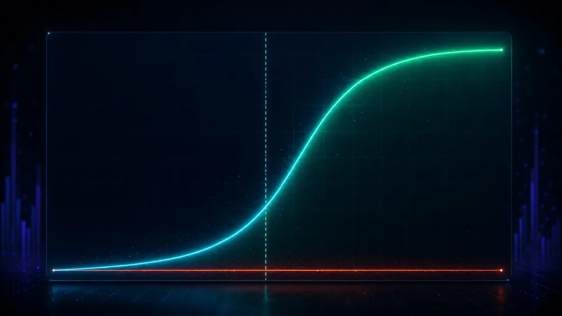
Plant one. In a field of 1,000 strategies, make 25 of them carry a real edge of known strength and leave the rest as noise, then run the search and ask whether DSR flags the winner. Sweep the planted edge from weak to strong and the detection power traces a clean S-curve (false-positive rate held at ~0 throughout):
| Planted true Sharpe (annualized) | DSR detection power | DSR false-positive rate |
|---|---|---|
| 0.79 | 0.005 | 0.000 |
| 1.27 | 0.090 | 0.000 |
| 1.90 | 0.651 | 0.000 |
| 2.54 | 0.998 | 0.000 |
| 3.17 | 1.000 | 0.000 |
Look at where the curve turns. Below the noise ceiling — a true annualized Sharpe of 0.79, well under 1.63 — DSR fires 0.5% of the time, correctly refusing to call it: an edge that weak is genuinely indistinguishable from the luck a 1,000-trial search generates, and pretending otherwise would be dishonest, not powerful. Right around the ceiling the curve climbs steeply (0.09 at 1.27, 0.65 at 1.90). By an annualized Sharpe of 2.54 the power is 0.998; by 3.17 it is a perfect 1.000. Strong edges are retained essentially every time, false positives stay pinned to zero, and the 50%-power crossover sits at an annualized Sharpe of about 1.73 (derived by interpolation between the 1.27 and 1.90 rows) — just above the 1.63 noise ceiling, exactly where an honest bar should put it: the point where an edge starts to outrun what a 1,000-trial search invents.
That is the property you actually want, stated as an S-curve: edges below the noise ceiling are correctly ruled out as luck; edges comfortably above it are kept with power approaching one. The naive test, for contrast, "detects" the planted edge 67% of the time even at a true Sharpe of 0.79 — but that number is meaningless, because we already saw it detects a non-existent edge 100% of the time. A test that fires on everything has no power; it has no discrimination. DSR trades a little sensitivity to marginal edges (the 0.79 and 1.27 rows) for the thing that matters: its discoveries are real.
Act 5 — The practitioner's trap: correlated grids

Everything so far used independent strategies — the cleanest possible setting, and the one where DSR's independence assumption holds exactly. Real parameter grids are not like that, and this is where a tool used naively becomes a new way to be wrong.
Take an honest moving-average crossover search: 16 fast lengths 40 slow lengths trials, each 755 observations. A grid like this is drenched in correlation — fast=45/slow=120 and fast=45/slow=125 are almost the same strategy, so their return streams move together. Measured average pairwise correlation across the 640 trials: about 0.61. Those are not 640 independent bets. Not remotely.
Case A — random walk (no edge): every method kills it, correctly
Run the grid on a pure random walk. The winner looks tempting: params fast=45/slow=120, best annualized Sharpe 0.81, single-test p-value 0.081. Every method sees through it:
| Method | Result | Verdict |
|---|---|---|
| DSR (raw K = 640) | 0.431 | reject (< 0.95) |
| Reality Check p | 0.570 | reject |
| SPA-type p (studentized RC) | 0.569 | reject |
| Harvey-Liu haircut | 100% | reject |
Start with the tell that needs no deflation at all: even the un-adjusted finite-sample significance of this winner, -vs-zero, is only 0.918 — already short of 0.95 before we correct for a single one of the 640 trials. Deflation then buries it: the bar is a per-observation , an annualized ~0.91 (derived: ) — above the winner's 0.81. The best strategy doesn't even reach the noise ceiling, DSR ≈ 0.43 (worse than a coin flip), and Reality Check, the SPA-type test, and a 100% haircut all agree: nothing here. Perfect. This is the easy case, and it works — and, as we will see, it stays rejected at every effective-trial count we try.
Case B — a genuine regime edge: the raw DSR gets it wrong
Now run the same grid on a regime-switching series that carries a real, exploitable edge. The winner is emphatic: params fast=3/slow=55, best annualized Sharpe 3.92 — this is the in-sample, selected Sharpe, itself selection-inflated by the search (not a true or out-of-sample edge), but the underlying regime effect is genuine — with a single-test p-value of and un-deflated significance -vs-zero of essentially 1.000. There is a real edge here and the winner found it. Watch the raw DSR reject it anyway:
| Method | Result | Verdict |
|---|---|---|
| DSR (raw K = 640) | 0.748 | reject (< 0.95) ✗ over-deflated |
| Reality Check p | 0.0024 | confirm ✓ |
| SPA-type p (studentized RC) | 0.0038 | confirm ✓ |
| Harvey-Liu haircut | 15% | confirm ✓ |
The raw DSR of 0.748 is a false rejection of a genuine edge. The reason is the independence assumption, now violated hard: DSR built its deflated bar by treating 640 correlated trials as 640 independent draws, which inflates the expected-maximum to a per-observation 0.221 — annualized ~3.51 (derived: ). Against a bar of 3.51, a winner of 3.92 clears it only modestly, and DSR lands at 0.748 — short of 0.95. Two things pump that bar up: the raw count (640 looks instead of a handful of effective ones), and genuine skill dispersion among the trials — some parameter pairs really are better on a regime series, which widens and lifts beyond what pure luck alone would. Both push the same way, and the bar ends up too high because the search was never really 640 independent looks; it was a few independent bets, sampled 640 times over.
Feed DSR the effective number of trials instead. The one-liner used above is a crude estimate from the average pairwise correlation:
def effective_n_trials(returns_matrix):
    """N_eff = N / (1 + (N-1) * rho_bar), clipped to [1, N].
    Correlated trials -> fewer independent bets."""
    C = np.corrcoef(returns_matrix, rowvar=False)
    rho_bar = max(np.nanmean(C[np.triu_indices(C.shape[0], k=1)]), 0.0)
    N = returns_matrix.shape[1]
    neff = N / (1.0 + (N - 1) * rho_bar)
    return float(min(max(neff, 1.0), N))
With and , this collapses the grid to an effective trials (derived: ), and the DSR jumps to 1.000. But stop before you celebrate that number, because it is the weakest evidence in this whole section. At the deflated bar collapses to an annualized — essentially the trial mean, essentially zero. Deflation there is switched off: DSR at is just re-reporting the winner's un-deflated finite-sample significance (-vs-zero ). The verdict is inherited from raw significance, not produced by the multiple-testing correction. And the mirror-image caveat on the random-walk side: its rejection at holds only because that winner was independently marginal to begin with (-vs-zero ). Anchor the whole argument on 1.6 and a skeptic is right to shrug: you turned the correction off and reported whatever was underneath.
So don't anchor on one estimator. The honest move — and the stronger one — is to compute five different standard ways and read the verdict across the whole band. Here are five estimators applied to the same 640-trial signal grid, each with the deflated bar it implies and the DSR it produces:
| Effective-trial estimator | Deflated bar (annual) | DSR | Verdict | |
|---|---|---|---|---|
| Average correlation | 1.6 | 0.25 | 1.000 | retain |
| Participation ratio | 2.4 | 0.43 | 1.000 | retain |
| PCA (95% of variance) | 16 | 1.85 | 1.000 | retain |
| Kaiser (eigenvalues > 1) | 21 | 2.00 | 0.999 | retain |
| Cheverud-Nyholt | 370 | 3.31 | 0.845 | reject |
| raw grid count (no adjustment) | 640 | 3.51 | 0.748 | reject |
Estimators: average correlation is the one-liner above; participation ratio and the PCA-95%/Kaiser counts read the effective dimensionality off the correlation matrix's eigenvalues; Cheverud-Nyholt is a variance-of-eigenvalues estimator from the genetics literature that is known to over-count under near-equicorrelation.
Now the point lands, and it is not "any adjustment saves you." Look at the defensible middle — PCA-95% () and Kaiser (). These are not the deflation-is-off regime; they impose a real annualized bar of 1.85 to 2.00 — a serious haircut, well above the noise, a genuine multiple-testing penalty for 16-21 effective looks. And the 3.92 edge still clears it (DSR 1.000 and 0.999). The signal survives DSR for any below 144.8 (derived from the crossing point); it fails only under Cheverud-Nyholt's , an estimator that provably over-counts when trials are near-equicorrelated — and even the raw, unadjusted count of 640 only pushes DSR down to 0.748, not to zero. The random-walk winner, run through the exact same five estimators, is rejected at every one of them (it survives for no above 1). That is the real result: not a single lucky number, but a verdict that is stable across the entire band of standard effective-trial estimates — which is far stronger evidence than trusting any one of them.
One technical caveat on the crudest estimator, because it explains why it sits at the soft end: is really the variance-reduction factor for the mean of correlated variables (how much averaging buys you under correlation ). DSR's benchmark is an extreme-value quantity — the expected maximum of the trials — so using a mean-variance shrinkage as its trial count is a functional mismatch: right in direction (correlated ⇒ fewer effective trials), but not the quantity the maximum's distribution actually depends on. That is exactly why the eigenvalue-based estimators in the middle of the band are the more trustworthy read, and why the band, not the point, is the deliverable.
The lesson: use both tools, and feed DSR the right N

Two things fall out of Case B, and both are load-bearing:
- The raw grid size is the wrong N for DSR whenever trials are correlated — and no single effective-N is the right one either. Plugging 640 into a formula that assumes independence over-deflates: it manufactures a noise ceiling far taller than the search actually reached and buries real edges under it. DSR needs the effective trial count — but the fix is not to trust one estimator (least of all the crudest, where the correction switches off near ). It is to read the verdict across the whole band of standard estimators (here 1.6 to 370) and see whether it is stable. For this edge it was: retained everywhere the deflation is genuinely active (a real 1.85-2.00 annual bar at -), failing only under an estimator that over-counts. A stable-across-the-band verdict is far stronger than any single number.
- Pair DSR with a Reality Check. Notice that the Reality Check and its SPA-type (studentized) cousin got Case B right without any trial-count surgery at all (p = 0.0024 and 0.0038) — they handle dependence natively, through the stationary bootstrap, because they resample the actual correlated return streams instead of counting hypothetical independent bets. That is the tie-breaker for the whole effective-N mess: RC needs no . DSR and RC answer different questions: DSR asks "is the winner special within this search?" (and needs to know how many effective looks the search took); RC/SPA-type ask "does the best rule beat cash after data-snooping?" (and read the dependence off the data itself). You want both. When they disagree — as the raw-count DSR and RC did here — the disagreement is diagnostic: it usually means your is wrong.
This is the same structural warning our speed-ladder and IPC-tax studies kept hitting from the engineering side — a fast search that runs a huge correlated grid is not buying you a huge number of independent bets, and treating grid size as trial count fools both your optimizer and your significance test. The forthcoming companion on the probability of backtest overfitting attacks the same selection bias from the resampling side (CSCV), and pairs naturally with everything here: DSR prices the winner, PBO prices the procedure.
Honesty notes
Three caveats, stated plainly, because the whole point of a controlled study is to not oversell it.
- The returns are synthetic. iid Normal for the calibration and power experiments, a regime-switching process for the genuine-edge case — chosen for controlled ground truth, not for market realism. Real returns are fat-tailed, autocorrelated, and non-stationary, and PSR's skew/kurtosis terms exist precisely to handle the first of those. The deliverable here is the calibrated method, not a strategy: we can only prove a test controls false discoveries by running it on data where we know there is nothing to discover. That requires manufacturing the ground truth.
- No effective-N estimator is canonical — which is why we reported five. The average-correlation one-liner is reviewer-legible and directionally right (more correlation ⇒ fewer effective trials), but it is the variance-reduction factor for a mean — a functional mismatch with DSR's maximum benchmark — and near it switches the deflation off entirely. The eigenvalue estimators (participation ratio, PCA-95%, Kaiser) are better matched but still heuristic, and Cheverud-Nyholt over-counts under equicorrelation. The fuller, principled approach is trial clustering (Bailey & López de Prado's DSR Appendix 3): group trials by correlation structure and count clusters rather than collapsing everything to one scalar. We report the whole band precisely because the choice is not settled — a verdict stable across all five estimators is the honest claim; one that depended on picking a single estimator would not be.
- The bootstrap is a studentized Reality Check, not the full Hansen SPA, and resample counts differ by experiment. Wherever this article says "SPA-type," it means White's Reality Check with per-rule studentization; Hansen's full consistent, sample-dependent recentering is not implemented. The calibration false-discovery rates use 500 stationary-bootstrap resamples per search across 400 searches; the two case-study RC/SPA-type p-values use 5,000 resamples each. Average block length 20 throughout (Politis-Romano), , 252 periods/year for annualization. Change these and the third-decimal numbers move; the story — naive 1.000 versus principled 0.001-0.057, an S-curve reaching 50% power just above the noise ceiling, and a correlated-grid trap whose verdict must be read across the effective-N band — does not.
Takeaways
- A parameter search is a multiple-testing machine, and the naive significance test is blind to it. On 1,000 zero-edge strategies the best annualized Sharpe averages 1.63 with a single-test p-value median of 0.000686 — and the "is it significant?" test declares a discovery 100% of the time (false-discovery rate 1.000). A great Sharpe from nothing, certified significant by a test that was never asking the right question.
- The Deflated Sharpe Ratio moves the goalpost from zero to the noise ceiling. DSR compares the winner not against zero but against , the expected best-by-luck of a search this size — which for the null case lands at an annualized 1.63, exactly where the average noise winner sits (derived: ). Its null false-discovery rate is 0.001; the Harvey-Liu haircut (Bonferroni/Holm 0.057, BHY 0.007) and White's Reality Check (0.022) reach the same control by other roads.
- It keeps the real edges. DSR's detection power traces an S-curve that reaches 50% power at an annualized Sharpe of ~1.73 — just above the 1.63 noise ceiling: 0.005 at a true annualized Sharpe of 0.79, 0.651 at 1.90, 0.998 at 2.54, 1.000 at 3.17, false positives ~0 throughout. Edges below the ceiling are correctly ruled indistinguishable from luck; edges above it are retained with power approaching one.
- Correlated grids break the raw DSR — and no single effective-N rescues it; the band does. On a 640-cell MA crossover (average pairwise correlation ~0.61), the raw-count DSR falsely rejected a genuine (in-sample selected, annual 3.92) edge (0.748 < 0.95) because 640 correlated trials are not 640 independent bets. But the fix is not one magic — at the crudest estimate () the deflation is essentially switched off (bar ~annual 0.25) and DSR merely echoes raw significance. The real evidence is that the edge is retained across the whole band of standard estimators — DSR 1.000/1.000/1.000/0.999 at 1.6/2.4/16/21, including a genuine annual bar of 1.85-2.00 at the defensible PCA-95%/Kaiser mid-range — surviving for any , and failing only under Cheverud-Nyholt's over-counting 370. The random walk is rejected at every estimator. Read the band, not a point.
- Pair DSR with a Reality Check, because they answer different questions. The Reality Check and its SPA-type (studentized) cousin confirmed the real edge (p = 0.0024 and 0.0038) with no trial-count surgery — they handle dependence natively through the stationary bootstrap, which is exactly the tie-breaker when the effective-N is contested. DSR asks "is the winner special within this search?"; RC/SPA-type ask "does the best beat cash after data-snooping?" A disagreement between them is a signal your is wrong. Run both.
The winner of a search is guilty until proven innocent. The naive p-value is not a proof of innocence — it is the search's own inflated testimony, and it will vouch for pure noise with twelve zeros of confidence. Deflate the benchmark to what luck delivers, count your effective trials honestly, and bootstrap the max for a second opinion. What clears all three bars might actually be real. What clears only the naive one is the tallest of a thousand coin-flippers.
The full experiment — the null-calibration harness, the planted-edge power sweep, the correlated-grid searches, and every number in this article regenerable from one deterministic script — is in the companion paper at deflated-sharpe.marketmaker.cc, with code and data at github.com/suenot/deflated-sharpe-search.
Authors

Trading-systems engineer
Trading-systems engineer building bots since 2017: cross-exchange arbitrage (connected up to 30 venues), cointegration-based pairs arbitrage across spot and futures, scalping, news and sentiment-driven strategies, trend algorithms, and portfolio management and balancing algorithms. Also builds sub-millisecond order execution, big-data warehouses, backtesting engines, AI agents, and trading interfaces (incl. open-source profitmaker.cc). Stack: JS/TS, Python, Rust/Zig/Go, DevOps, backend, frontend, architecture.
Read More

The Probability of Backtest Overfitting: Did Your Search Beat a Coin Flip?

Objective-Function Design: The Metric You Optimize Secretly Picks Your Strategy