Нейронные ОДУ: превосходит ли непрерывное время функцию дельта-времени?

Нейронные обыкновенные дифференциальные уравнения (Чен и др., NeurIPS 2018) параметризуют производную скрытого состояния с помощью нейронной сети и позволяют решателю ОДУ вычислить выходные данные. Модель становится непрерывной по глубине и, что более полезно для рынков, непрерывной во времени: скрытое состояние может быть оценено в любой момент , а не только в точках сетки, в которых находятся ваши данные.
Это свойство явно подходит для финансовых данных, которые поступают через случайные промежутки времени. Но за этим заявлением скрывается гораздо более слабое утверждение, чем кажется. Простое ГРУ предоставило дополнительную функцию ввода — с момента предыдущего наблюдения — тоже "знает", сколько времени прошло. Реальный вопрос не в том, могут ли модели с непрерывным временем принимать нерегулярные данные. Вопрос в том, сможет ли изученная непрерывная динамика между наблюдениями извлечь что-то, что функция дельты времени еще не дает вам, за цену в десять-сотню раз превышающую стоимость вывода.
В этой статье описан эксперимент, приведена полная цепочка инструментов для его проведения и указано, что должно показать сравнение, чтобы оправдать это усложнение. Сторона аргумента, связанная с построением баров — что время торговли само по себе несет сигнал — подтверждена измерениями для 17 типов баров в статье за пределами временных баров; здесь важно лишь следствие для модели: решатель вычисляет скрытое состояние в произвольный момент , поэтому интерполяция или дополнение не нужны.
Тестируемое заявление
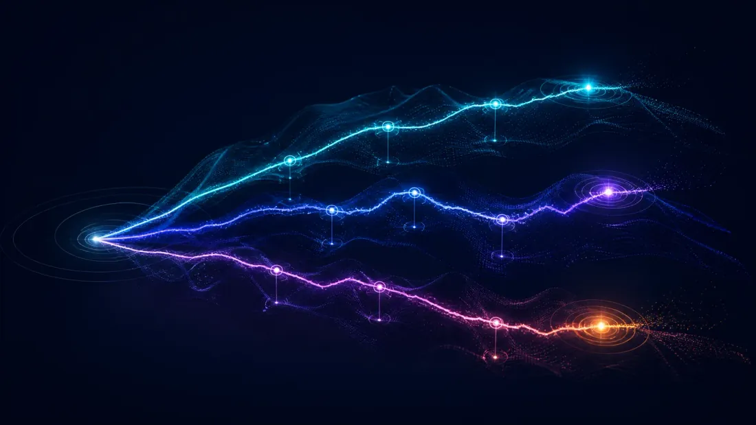
Три вложенные гипотезы, каждая из которых строго сильнее предыдущей:
- H1 — соответствие ODE-RNN необработанному нерегулярному торговому потоку BTC превосходит соответствие GRU тому же потоку вообще без информации о времени. Это почти наверняка и почти бесполезно: ODE-RNN просто располагает информацией, которой не хватает базовой линии.
- H2 — ODE-RNN превосходит ту же GRU, когда GRU получает в качестве входного признака. Это честный тест. Именно это утверждение обычно подразумевается в литературе о Neural ODE, но на финансовых данных его почти никогда не демонстрируют.
- H3 — преимущество H2 сохраняется в рамках бюджета задержки, то есть ODE-RNN развертывается с решателем с фиксированным шагом, достаточно быстрым для работы в реальном времени, а не с адаптивным
dopri5.
Протокол эксперимента
Тот же тиковый поток, та же цель, одинаковый бюджет настройки для обоих вариантов. Никакой повторной выборки до минутных баров — она разрушает точную структуру, которую мы проверяем.
| Параметр | |
|---|---|
| Данные | Торговые распечатки BTC, переменное время между поступлениями, без повторной выборки |
| Варианты | ODE-RNN; GRU + ; GRU без временного признака |
| Цель | Одинакова для всех вариантов; задается вместе с обучением |
| Метрики | RMSE, удержанное логарифмическое правдоподобие, настенные часы на эпоху, задержка вывода на каждый шаг |
| Развертка решателя | dopri5 (rtol 1e-5) против Эйлера с фиксированным шагом, сопоставленные по точности обучения |
| Разбиение | Скользящее тестирование вперед, только вне обучающей выборки |
| Вариант | RMSE | Лог-правдоподобие | с/эпоха | Задержка вывода/шаг |
|---|---|---|---|---|
| ГРУ (без временных характеристик) | — | — | — | — |
| GRU + log(dt) | — | — | — | — |
| ОДУ-РНН (допри5) | — | — | — | — |
| ОДУ-RNN (Эйлер с фиксированным шагом) | — | — | — | — |
Отрицательный результат H2 вполне можно публиковать, и он, возможно, даже ценнее положительного — тот же стандарт применен в статье честный отрицательный результат и в материале о дефлированном коэффициенте Шарпа при множественном тестировании.
Вторичный эксперимент: CNF против Student-t
Если сравнение ODE-RNN слишком дорогое, более дешевый эмпирический якорь является распределительным: подберите непрерывный нормализующий поток к реальной ежедневной доходности BTC и сравните его подобранную плотность с аппроксимацией Стьюдента и с эмпирическим хвостом, сообщая об ошибках хвостового квантиля на уровнях 1% и 5%. Это напрямую связано с распределительной работой, уже измеренной в Прогнозирование волатильности GARCH и асимметричный ГАРЧ.
Остальная часть этой статьи — это предыстория и набор инструментов, необходимых для запуска вышеописанного.
Предыстория: от ResNets к непрерывной динамике

Остаточная сеть вычисляет . Уменьшите размер шага и увеличьте количество слоев, и вы приблизитесь к непрерывному пределу:
Вместо дискретных слоев с отдельными параметрами единая сеть определяет мгновенную скорость изменения. Выход в момент решает задачу начального значения:
Решатель "черного ящика" (Эйлер, Рунге-Кутта, Дорманд-Принс) вычисляет интеграл численно, адаптивно выбирая размеры шага на основе локальных оценок ошибок.
Сопряженный метод
Обратное распространение ошибки на каждом шаге решателя сохраняет все промежуточные состояния, тратя память пропорционально количеству шагов. Чен и др. вместо этого решите обратную ОДУ с помощью память. Определить присоединенное состояние , что удовлетворяет
и накапливаем градиент параметра вдоль обратного прохода:
Обратный проход решает расширенную систему, одновременно вычисляя , и , запуская решатель в обратном порядке от к .
Компромисс: реконструкция при обратном проходе накапливает числовую ошибку, особенно для жесткой или хаотичной динамики. Чекпойнтинг — золотая середина: сохраняйте в нескольких промежуточных моментах и пересчитывайте состояние между ними. Ценовые процессы являются непрерывными полумартингалами и умеренно гладкими, поэтому сопряженный метод обычно работает; жесткость вокруг событий микроструктуры может потребовать адаптивных решателей или гибридов.
ODE-RNN: непрерывное скрытое состояние между наблюдениями

ODE-RNN — это архитектура, которую включает основной эксперимент. Между наблюдениями скрытое состояние развивается согласно ОДУ:
Когда наблюдение прибывает в , запускается дискретное обновление:
Верхние индексы обозначают состояние непосредственно перед наблюдением и сразу после него. Между наблюдениями работает изученная непрерывная динамика, а в моменты наблюдений поступает новая информация.
Механизм, который проверяет абляция H2, таков: длинный промежуток означает, что скрытое состояние сильно изменилось под действием — затухая к базовой линии или расходясь, — и форма этой эволюции изучается, а не задается одним числом. Окупается ли эта выразительность на реальных торговых данных, пока не измерено.
Естественные соответствия, выходящие за рамки тиков: портфели с несколькими активами, где каждый актив имеет свой собственный график наблюдения, а скрытое состояние коррелирующих активов продолжает развиваться, в то время как наблюдается только один; и сигналы, обусловленные событиями (новости, доходы, макро-релизы), поступающие в нерегулярное время.
Нейронные SDE: добавление стохастических компонентов

Нейронные ОДУ детерминированы и не могут представить шум в траектории цены. Классический подход — геометрическое броуновское движение, нейтральный к риску дрейф и то, как предположения о постоянной волатильности терпят неудачу на фоне улыбки, — описан в статье о ценообразовании опционов Блэка — Шоулза. Нейронные СДУ заменяют параметрическую форму изученным диффузионным членом:
это дрейф, диффузия, Винеровский процесс, оба и нейронные сети.
Архитектура: дрейфовая сеть и диффузионная сеть
- Дрифтерная сеть : ожидаемая траектория — тренд, возврат к среднему значению, импульс. Обучены минимизировать ошибку прогнозирования.
- Диффузионная сеть : величина шума, изученная как функция состояния. Высокий при нестабильных режимах, низкий при спокойных.
Раскол отражает классические квантовые финансы: дрейф — это нейтральная к риску (или P-мера) динамика, диффузия — это поверхность волатильности.
Обучение нейронных SDE
Стохастический интеграл не является классически дифференцируемым. Три подхода:
- Градиенты по путям: трюк с перепараметризацией — выборка броуновских путей, дифференцирование с помощью решателя, рассматривающего шум как фиксированный входной сигнал.
- Сопоставление баллов: оценка и обучать с помощью целей шумоподавления — тот же механизм, который используется в качестве автономной генеративной модели в диффузионные модели для криптопрогнозирования, здесь понижен до варианта обучения для SDE.
- Сопоставление конечномерного распределения: сопоставьте маргинальные значения во время наблюдения, а не меры полного пути.
Pathwise — это практическое значение по умолчанию. torchsde реализует Эйлера-Маруяму, Мильштейна и стохастический метод Рунге-Кутты с поддержкой автодифференциации.
Изучение поверхности волатильности
Классические модели (Хестон, SABR) накладывают параметрические формы на коэффициент диффузии. Нейронное SDE учится как произвольная функция:
Это универсальный аппроксиматор диффузионных процессов — любого процесса Ито с произвольной точностью при достаточной мощности.
Скрытые ODE для отсутствующих и асинхронных данных

Скрытая ОДУ (Рубанова, Чен, Дювено, 2019) объединяет нейронную ОДУ с VAE: финансовые ряды представляют собой зашумленные наблюдения плавного основного процесса, изученного в низкомерном скрытом пространстве.
- Сеть распознавания: ODE-RNN, проходящая в обратном направлении через наблюдения для получения .
- Скрытая динамика: .
- Декодер: , доступный для оценки в любое запрошенное время.
Проигрыш стандартный ELBO:
Оценка состояния портфеля: на основе редких асинхронных наблюдений за активами можно сделать вывод о непрерывном скрытом состоянии, фиксирующем совместную динамику — по сути, это нелинейная, обученная версия фильтра Калмана.
Вменение отсутствующих данных: остановки и перерывы в выходные дни приобретают плавно интерполированную скрытую траекторию; декодер создает вероятные пути через зазор с неопределенностью из-за задней части VAE.
Многочастотное объединение: дневные закрытия, внутридневные VWAP и тиковые данные в одной модели без общей временной сетки.
Непрерывные нормализующие потоки для обратных распределений
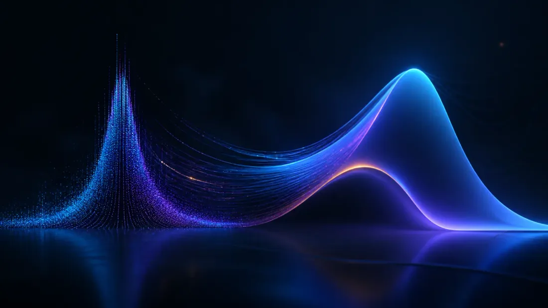
CNF используют Neural ODE для преобразования простого базового распределения в сложную цель. Преобразование , а логарифмическая плотность соответствует мгновенному изменению переменных:
Интегрируйте состояние и логарифм плотности вперед от , чтобы получить и . След якобиана оценивается с помощью стохастической оценки Хатчинсона, что обеспечивает масштабируемость.
Доходность криптовалюты имеет высокую эксцессивность и отрицательную асимметрию — это измерено на реальных данных в материалах о прогнозировании волатильности GARCH и асимметричном GARCH и эффекте рычага — и CNF изучает эту форму, а не задает ее заранее. Условное представление потока через переменные состояния позволяет форме меняться вместе с режимом. Поскольку плотность точна, а не приближена, ее можно передать в хвостовые метрики из монте-карло и бутстрэп-бэктестов и расчет CVaR в портфельном конвейере HRP/CVaR; совместная структура хвостов обрабатывается отдельно в копульных моделях совместного риска.
Условная оценка плотности
Полезная формулировка — это прямое сравнение трех опубликованных подходов к одной проблеме. TFT дает фиксированный набор квантилей из выходного слоя. Конформное предсказание дает калиброванные интервалы с гарантией покрытия. Условный CNF дает точную дифференцируемую плотность:
Отличительным свойством является дифференцируемость: плотность может находиться внутри следующей цели и распространяться обратно, что не поддерживается ни фиксированными квантилями, ни конформными интервалами. Здесь не проверялось, стоит ли точная плотность своих затрат по сравнению с квантилями TFT для той же цели.
Сравнение с дискретными альтернативами
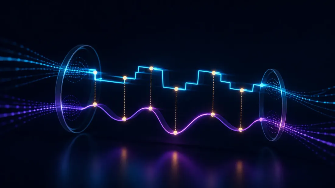
| Свойство | ЛСТМ/ГРУ | Трансформатор | Нейронная ОДУ | Нейронное СДУ |
|---|---|---|---|---|
| Работа с нерегулярным временем | Плохо (нужно дополнение) | Позиционное кодирование | Встроенная | Встроенная |
| Память (тренировка) | примыкающий | примыкающий | ||
| Количественная оценка неопределенности | Нет (детерминированная) | Нет (детерминированная) | Через ансамбли | Встроенная |
| Интерполяция между наблюдениями | Нет | Нет | Да | Да |
| Плотность непрерывного времени | Нет | Нет | Через CNF | Через измерение пути |
| Стоимость вычислений | Низкий | Умеренный | Переменная (решатель) | Высокий (решатель SDE) |
Половина этой таблицы, посвященная LSTM-вниманию, подробно обсуждается с контрольными показателями в разделе TFT-статья - см. разделы "TFT против LSTM против ванильного трансформатора" и "Когда LSTM все еще побеждает". Новые столбцы здесь — это два справа, а строки, отвечающие на вопросы H2/H3, — это две последние.
Реализация Python с помощью torchdiffeq
torchdiffeq предоставляет решателям ОДУ сопряженное обратное распространение ошибки.
Базовая нейронная ОДУ для динамики цен
import torch
import torch.nn as nn
from torchdiffeq import odeint_adjoint as odeint

class PriceDynamics(nn.Module):
    """Neural network defining dh/dt = f(h, t)."""

    def __init__(self, hidden_dim: int = 64):
        super().__init__()
        self.net = nn.Sequential(
            nn.Linear(hidden_dim, 128),
            nn.Tanh(),
            nn.Linear(128, 128),
            nn.Tanh(),
            nn.Linear(128, hidden_dim),
        )

    def forward(self, t, h):
        return self.net(h)


class NeuralODEPredictor(nn.Module):
    """
    Encode observed features -> latent state,
    evolve via Neural ODE,
    decode to price prediction.
    """

    def __init__(self, input_dim: int, hidden_dim: int = 64):
        super().__init__()
        self.encoder = nn.Linear(input_dim, hidden_dim)
        self.dynamics = PriceDynamics(hidden_dim)
        self.decoder = nn.Linear(hidden_dim, 1)

    def forward(self, x0, eval_times):
        """
        x0:         (batch, input_dim) features at t=0
        eval_times: (T,) times at which to evaluate the ODE
        Returns:    (T, batch, 1) predictions
        """
        h0 = self.encoder(x0)                          # (batch, hidden_dim)
        h_traj = odeint(self.dynamics, h0, eval_times,
                        method='dopri5', rtol=1e-5, atol=1e-7)
        return self.decoder(h_traj)
ODE-RNN для нерегулярных тиковых данных
Это экспериментальное отделение. Базовый уровень, который он должен превзойти, составляет nn.GRUCell в одном потоке с log(t_next - t_prev) объединено с x.
class ODERNNCell(nn.Module):
    """Single step: ODE-evolve, then RNN-update."""

    def __init__(self, input_dim: int, hidden_dim: int = 64):
        super().__init__()
        self.dynamics = PriceDynamics(hidden_dim)
        self.gru_cell = nn.GRUCell(input_dim, hidden_dim)

    def forward(self, h, x, t_prev, t_next):
        times = torch.tensor([t_prev, t_next], dtype=torch.float32)
        h_evolved = odeint(self.dynamics, h, times,
                           method='dopri5')[-1]  # state at t_next
        h_updated = self.gru_cell(x, h_evolved)
        return h_updated


class ODERNN(nn.Module):
    """Process irregularly-sampled sequence."""

    def __init__(self, input_dim: int, hidden_dim: int = 64):
        super().__init__()
        self.cell = ODERNNCell(input_dim, hidden_dim)
        self.decoder = nn.Linear(hidden_dim, 1)
        self.hidden_dim = hidden_dim

    def forward(self, observations, times):
        """
        observations: list of (batch, input_dim) tensors
        times:        list of floats, observation timestamps
        """
        batch_size = observations[0].shape[0]
        h = torch.zeros(batch_size, self.hidden_dim)

        outputs = []
        for i in range(len(observations)):
            t_prev = 0.0 if i == 0 else times[i - 1]
            h = self.cell(h, observations[i], t_prev, times[i])
            outputs.append(self.decoder(h))

        return torch.stack(outputs)  # (seq_len, batch, 1)
Тренировочный цикл
def train_neural_ode(model, train_loader, epochs=100, lr=1e-3):
    optimizer = torch.optim.Adam(model.parameters(), lr=lr)
    scheduler = torch.optim.lr_scheduler.CosineAnnealingLR(
        optimizer, T_max=epochs
    )

    for epoch in range(epochs):
        epoch_loss = 0.0
        for batch in train_loader:
            features, times, targets = batch
            optimizer.zero_grad()

            predictions = model(features, times)
            loss = torch.nn.functional.mse_loss(predictions, targets)

            loss.backward()
            torch.nn.utils.clip_grad_norm_(model.parameters(), max_norm=1.0)
            optimizer.step()

            epoch_loss += loss.item()

        scheduler.step()

        if (epoch + 1) % 10 == 0:
            avg_loss = epoch_loss / len(train_loader)
            print(f"Epoch {epoch+1}/{epochs}, Loss: {avg_loss:.6f}")
Непрерывный нормализующий поток для обратных распределений
from torchdiffeq import odeint

class CNFDynamics(nn.Module):
    """Dynamics for continuous normalizing flow."""

    def __init__(self, dim: int = 1, hidden_dim: int = 64):
        super().__init__()
        self.net = nn.Sequential(
            nn.Linear(dim + 1, hidden_dim),  # +1 for time
            nn.Tanh(),
            nn.Linear(hidden_dim, hidden_dim),
            nn.Tanh(),
            nn.Linear(hidden_dim, dim),
        )
        self.dim = dim

    def forward(self, t, state):
        z = state[..., :self.dim]
        t_expand = t.expand(z.shape[0], 1)
        zt = torch.cat([z, t_expand], dim=-1)
        dz = self.net(zt)

        e = torch.randn_like(z)
        e_dz = torch.autograd.grad(
            dz, z, e, create_graph=True
        )[0]
        trace_jac = (e_dz * e).sum(dim=-1, keepdim=True)

        return torch.cat([dz, -trace_jac], dim=-1)


class ReturnDistributionCNF(nn.Module):
    """Model return distributions with continuous normalizing flows."""

    def __init__(self, dim: int = 1):
        super().__init__()
        self.dynamics = CNFDynamics(dim)
        self.dim = dim

    def log_prob(self, x):
        """Compute log probability of observed returns."""
        log_p0 = torch.zeros(x.shape[0], 1)
        state0 = torch.cat([x, log_p0], dim=-1)
        state0.requires_grad_(True)

        times = torch.tensor([1.0, 0.0])  # backward
        state_T = odeint(self.dynamics, state0, times,
                         method='dopri5')[-1]

        z_T = state_T[..., :self.dim]
        delta_log_p = state_T[..., self.dim:]

        log_p_base = -0.5 * (z_T ** 2 + torch.log(
            torch.tensor(2 * torch.pi)
        )).sum(dim=-1, keepdim=True)

        return log_p_base + delta_log_p

    def sample(self, n_samples: int):
        """Generate samples from learned distribution."""
        z0 = torch.randn(n_samples, self.dim)
        log_p0 = torch.zeros(n_samples, 1)
        state0 = torch.cat([z0, log_p0], dim=-1)

        times = torch.tensor([0.0, 1.0])  # forward
        state_T = odeint(self.dynamics, state0, times,
                         method='dopri5')[-1]

        return state_T[..., :self.dim]
Практические заметки

Это то, что вас укусит во время эксперимента, описанного выше.
Выбор решателя и скорость
dopri5 дает гарантии точности, но переменные затраты на вычисления, поэтому H3 представляет собой отдельную гипотезу от H2: преимущество, которое существует только при использовании адаптивного решателя, может не выдержать живой бюджет задержки. Решатели с фиксированным шагом (Euler, RK4) обеспечивают предсказуемую задержку за счет точности. Практический компромисс: тренируйтесь с dopri5, разверните решатель с фиксированным шагом, откалиброванный для соответствия выходным данным адаптивного решателя на репрезентативных данных, и измерьте разрыв, а не предполагайте, что он небольшой.
odeint(f, h0, t, method='dopri5', rtol=1e-6, atol=1e-8)

odeint(f, h0, t, method='euler', options={'step_size': 0.1})
Для жестких задач вблизи прерывистых скачков method='implicit_adams' или method='scipy_solver'.
Численная стабильность
Если выводит большие значения, состояние расходится. Смягчения:
- Спектральная нормализация на слоях контролировать константу Липшица.
- Отсечение градиента во время обучения (показано в цикле обучения выше).
- Нормализация времени: масштабируйте временные метки до .
- Регуляризация по норме динамики: добавить к потере.
Интервал интеграции
Для данных, охватывающих несколько месяцев, не интегрируйте к минуты:
t_normalized = (timestamps - timestamps[0]) / (timestamps[-1] - timestamps[0])
Это сохраняет решатель в численно удобном режиме и делает изученную динамику масштабно-инвариантной. Это также имеет значение для сравнения: ненормализованная ODE-RNN может проигрывать базовой линии GRU по чисто численным причинам, что будет скорее артефактом измерения, чем результатом.
Обработка нескольких временных масштабов
Рынки имеют динамику в микросекундном, секундном, минутном и суточном масштабах одновременно, и одному нейронному ОДУ может быть сложно удержать их все. Опции: складывать несколько блоков ODE в разные временные масштабы; расширить скрытое измерение как для быстрой, так и для медленной емкости; или запускайте отдельные Neural ODE для каждой полосы частот и выходов предохранителей. (Это вопрос о возможностях модели, отличный от вопроса о достоверности бэктеста в детализация адаптивного разрешения.)
Открытые направления исследований
SDE Neural Jump: добавьте изученный компонент прыжка на случай внезапных сбоев (внезапных сбоев, неожиданностей в доходах):
где является компенсированной случайной мерой Пуассона и обученное ядро прыжка.
Дифференциальные уравнения, управляемые нейронами (нейронные CDE): замените винеровский процесс общим управляющим сигналом, позволяя наблюдаемым потокам данных управлять динамикой. Это естественно для потока ордеров, когда поток сделок и котировок управляет скрытым состоянием рынка.
Дифференцируемое рыночное моделирование: используйте нейронную SDE в качестве генеративной модели внутри дифференцируемого симулятора и комплексно тренируйте стратегии, осуществляя обратное распространение ошибки через сопряженное устройство. Стратегия и рыночная модель развиваются одновременно.
Нейронные ОДУ с учетом физики: PINN встраивают в потери невязку дифференциального уравнения — сама методика представлена в статья Навье-Стокса. Финансовое применение состоит в том, чтобы наложить условия отсутствия арбитража, паритета пут-колл и мартингейла в качестве штрафных санкций или жестких ограничений на изученную динамику.
Заключение

Модель непрерывного времени структурно правильна: рынки — это непрерывные процессы, наблюдаемые в дискретные, нерегулярные моменты времени, и модели должны это учитывать. Инструментальная цепочка зрелая — torchdiffeq, torchsde, в остальном простой PyTorch — и известные затраты — это скорость решателя и численная стабильность в течение длительных интервалов интегрирования.
Что не установлено, так это часть, которая решает, принадлежит ли что-либо из этого производственному стеку. Структурная правильность не является свидетельством предсказательного преимущества, а является конкретным преимуществом, заявленным для непрерывной динамики по сравнению с Эта функция здесь не измерялась на реальных торговых данных. Пока таблица H2 выше не заполнена, рассматривайте все, что находится ниже, как четко сформулированную гипотезу с прикрепленной работающей реализацией, а не как результат.
Ссылки
- Чен, RTQ, Рубанова, Ю., Бетанкур, Ж., Дювено, Д. (2018). Нейронные обыкновенные дифференциальные уравнения. НейрИПС 2018. arXiv:1806.07366
- Рубанова Ю., Чен RTQ, Дювено Д. (2019). Скрытые ОДУ для временных рядов с нерегулярной выборкой. НейрИПС 2019. arXiv:1907.03907
- Цзя Дж., Бенсон А.Р. (2019). Стохастические дифференциальные уравнения нейронного скачка. НейрИПС 2019.
- Киджер П., Моррилл Дж., Фостер Дж., Лайонс Т. (2020). Дифференциальные уравнения, управляемые нейронами, для нерегулярных временных рядов. НейрИПС 2020.
- Хасан А., Перейра Ж.М., Фарсиу С., Карин Л. (2021). Модели стохастических дифференциальных уравнений нейронных сетей с применением к прогнозированию финансовых данных. arXiv:2111.13164
- торчдиффек: github.com/rtqichen/torchdiffeq
- Учебные пособия по глубокому обучению UVA — нейронные ОДУ: uvadlc-notebooks.readthedocs.io
Авторы
Инженер торговых систем
Разработка торговых ботов с 2017 года: межбиржевой арбитраж (подключал до 30 бирж), парный арбитраж на коинтеграции между спотом и фьючерсами, скальпинг, фронтраннинг, торговля по новостям, сентиментный анализ, трендовые алгоритмы, а также алгоритмы управления и балансировки портфелей. Делает выставление ордеров до 1 мс, warehouse для big data, бэктестинг-движки, AI-агентов и интерфейсы для ботов (в т.ч. open-source profitmaker.cc). Стек: JS/TS, Python, Rust/Zig/Go, DevOps, backend, frontend, архитектура.
Читайте также

Hamiltonian Neural Networks: Does a Financial System Conserve Anything?

Trade Classification When You Have No Side Flag: Tick, Quote, Lee-Ready, BVC