Disclaimer: The information provided in this article is for educational and informational purposes only and does not constitute financial, investment, or trading advice. Trading cryptocurrencies involves significant risk of loss.
Subscribe to our newsletter for exclusive AI trading insights, market analysis, and platform updates.
Minute candles are the standard granularity for backtests. But within a single minute candle, price can move differently: sometimes by 0.01%, other times by 2%. When both stop-loss and take-profit fall within the [low, high] range of a single minute candle, the backtest doesn't know which triggered first. This is the fill ambiguity problem.
The naive solution is to switch to second-level data for the entire backtest. But over two years, that's ~63 million second bars instead of ~1 million minute bars. Storage increases 60x, speed drops proportionally.
Adaptive drill-down solves this problem: use fine granularity only where it's actually needed.
The Problem: Fill Ambiguity on Large Candles
Consider a specific situation. The strategy opened a long at 3000 USDT. Stop-loss: 2970 (-1%). Take-profit: 3060 (+2%).
The minute candle at 14:37:
Open: 3010
High: 3065
Low: 2965
Close: 3050
Both SL (2970) and TP (3060) fall within the range [2965, 3065]. Which triggered first?
Possible outcomes:
Price went down first -> SL triggered -> loss of -1%
Price went up first -> TP triggered -> profit of +2%
The difference in a single trade: 3 percentage points. With 10x leverage — 30%. For a backtest with hundreds of trades, incorrect fill ambiguity resolution systematically distorts results.
How Frameworks Handle This by Default
Most backtest engines use one of two heuristics:
Optimistic: TP triggers first -> inflated results
Pessimistic: SL triggers first -> deflated results
Both approaches are guesswork. Real data is available at second or even millisecond level, and there's no reason to guess when you can look.
Drill-Down: Three-Level Strategy
The drill-down idea: start at the minute level and "drill down" to a lower level only when there's ambiguity.
Level 1: 1m (minute candles)
  -> If SL or TP is unambiguously outside the [low, high] range — resolve on the spot
  -> If both are within the range — drill down

Level 2: 1s (second candles)
  -> Load 60 second bars for this minute
  -> Walk through second by second: which triggered first?
  -> If a second bar is also ambiguous — drill down

Level 3: 100ms (millisecond candles)
  -> Load up to 10 bars of 100ms for this second
  -> Resolve the fill at order book level
When Drill-Down Is Not Needed
In 95% of cases, drill-down is not required. Typical scenarios:
Unambiguous SL: candle high doesn't reach TP, low breaks through SL -> SL triggered, no drill-down needed.
Unambiguous TP: low doesn't reach SL, high breaks through TP -> TP triggered, no drill-down needed.
Neither triggered: both levels are outside the range -> position remains open.
Gap detection: the open of the next candle jumps through SL or TP -> execution at open price, no drill-down.
Drill-down is needed only for ~5% of bars — when both levels fall within the range of a single candle.
classAdaptiveFillSimulator:
"""
Three-level drill-down for determining fill order.
"""def__init__(self, data_loader):
self.loader = data_loader
self.cache_1s = {} # Cache of second data by monthdefcheck_fill(self, timestamp, candle_1m, sl_price, tp_price, side):
"""
Checks whether SL or TP triggered on the given minute candle.
Returns: ('sl', fill_price) | ('tp', fill_price) | None
"""
low, high = candle_1m['low'], candle_1m['high']
open_price = candle_1m['open']
if side == 'long':
if open_price <= sl_price:
return ('sl', open_price)
if open_price >= tp_price:
return ('tp', open_price)
else:
if open_price >= sl_price:
return ('sl', open_price)
if open_price <= tp_price:
return ('tp', open_price)
sl_hit = self._level_hit(sl_price, low, high, side, 'sl')
tp_hit = self._level_hit(tp_price, low, high, side, 'tp')
if sl_hit andnot tp_hit:
return ('sl', sl_price)
if tp_hit andnot sl_hit:
return ('tp', tp_price)
ifnot sl_hit andnot tp_hit:
returnNonereturnself._drill_down_1s(timestamp, sl_price, tp_price, side)
def_drill_down_1s(self, minute_ts, sl_price, tp_price, side):
"""Level 2: second-by-second pass."""
bars_1s = self.loader.load_1s_for_minute(minute_ts)
if bars_1s isNoneorlen(bars_1s) == 0:
returnself._pessimistic_fill(side, sl_price, tp_price)
for bar in bars_1s:
sl_hit = self._level_hit(sl_price, bar['low'], bar['high'], side, 'sl')
tp_hit = self._level_hit(tp_price, bar['low'], bar['high'], side, 'tp')
if sl_hit andnot tp_hit:
return ('sl', sl_price)
if tp_hit andnot sl_hit:
return ('tp', tp_price)
if sl_hit and tp_hit:
result = self._drill_down_100ms(bar['timestamp'], sl_price, tp_price, side)
if result:
return result
returnself._pessimistic_fill(side, sl_price, tp_price)
def_pessimistic_fill(self, side, sl_price, tp_price):
"""Pessimistic assumption: SL for longs, TP for shorts."""if side == 'long':
return ('sl', sl_price)
else:
return ('sl', sl_price)
Performance
Mode
Time per fill check
When used
1m (no drill-down)
~0ms
~95% of cases
1s drill-down
~5ms (first access to month)
~5% of cases
100ms drill-down
~1ms
<0.5% of cases
Over a 2-year backtest with ~400 trades, drill-down is invoked for approximately 20 candles. Total overhead — less than 1 second for the entire backtest.
Adaptive Data Storage
Drill-down requires second and millisecond data. But storing everything at maximum granularity is impractical:
Granularity
Bars over 2 years
Parquet size
1m
~1.05M
~15 MB
1s
~63M
~550 MB/month
100ms
~630M
~5 GB/month
A complete 1s archive over 2 years is about 13 GB. 100ms — over 100 GB. Storing everything is possible but wasteful, considering that drill-down uses less than 1% of this data.
Hot-Second Detection
The key observation: seconds in which price moves significantly represent a small fraction. If price changed by less than 0.1% within a second — there's no point storing the 100ms breakdown for that second.
Hot-second detection: when downloading and processing data, we analyze each second and generate 100ms candles only for "hot" seconds — those where price movement exceeded the threshold.
defprocess_trades_adaptive(
trades: pd.DataFrame,
min_price_change_pct: float = 1.0,
) -> tuple[pd.DataFrame, pd.DataFrame]:
"""
Processes raw trades into an adaptive structure:
- 1s candles for all seconds
- 100ms candles only for "hot" seconds
Args:
trades: DataFrame with columns [timestamp, price, quantity]
min_price_change_pct: threshold for drill-down to 100ms
Returns:
(df_1s, df_100ms_hot) — second candles and 100ms for hot seconds
"""
trades['second'] = trades['timestamp'].dt.floor('1s')
df_1s = trades.groupby('second').agg(
open=('price', 'first'),
high=('price', 'max'),
low=('price', 'min'),
close=('price', 'last'),
volume=('quantity', 'sum'),
)
df_1s['price_change_pct'] = (df_1s['high'] - df_1s['low']) / df_1s['open'] * 100
hot_seconds = df_1s[df_1s['price_change_pct'] >= min_price_change_pct].index
hot_trades = trades[trades['second'].isin(hot_seconds)]
hot_trades['bucket_100ms'] = hot_trades['timestamp'].dt.floor('100ms')
df_100ms = hot_trades.groupby('bucket_100ms').agg(
open=('price', 'first'),
high=('price', 'max'),
low=('price', 'min'),
close=('price', 'last'),
volume=('quantity', 'sum'),
)
return df_1s, df_100ms
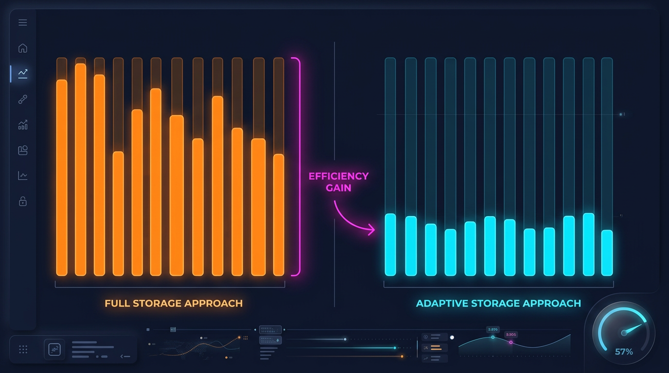
Storage Savings
For example — ETHUSDT over a typical month:
Approach
Size
Granularity
1m only
~1 MB
1 minute
All 1s
~550 MB
1 second
All 100ms
~5 GB
100 ms
Adaptive
~600 MB
1s + 100ms only for hot seconds
With a threshold of min_price_change_pct = 1.0%, hot seconds account for less than 1% of all seconds. 100ms data for them adds ~50 MB to the 550 MB of second data — a negligible overhead.
If second data is also stored adaptively (only when movement within a minute exceeds 0.1%), the volume can be reduced by another 3-5x.
DELTA_BINARY_PACKED for timestamps: consecutive timestamps differ by a fixed value (60 for 1m, 1 for 1s). Delta encoding compresses them to nearly zero.
BYTE_STREAM_SPLIT for float: splits float32 bytes into streams (all first bytes together, all second bytes together, etc.). For smoothly changing prices, this achieves 2-3x better compression than standard encoding.
ZSTD level 9: good compression with acceptable decompression speed.
float32 instead of float64: sufficient for prices and volumes, saves 50% memory.
Lazy Loading with Caching
Drill-down requests second data for a specific minute. Loading a parquet file for each request is slow. The solution — lazy loading with an LRU cache by month.
from functools import lru_cache
import pyarrow.parquet as pq
import pandas as pd
classAdaptiveDataLoader:
"""
Lazy loader with cache: loads second data by month,
keeps the last N months in memory.
"""def__init__(self, symbol: str, data_dir: str = "data", cache_months: int = 2):
self.symbol = symbol
self.data_dir = data_dir
self.cache_months = cache_months
self._cache_1s: dict[str, pd.DataFrame] = {}
defload_1s_for_minute(self, minute_ts: pd.Timestamp) -> pd.DataFrame | None:
"""Load 1s data for a specific minute."""
month_key = minute_ts.strftime("%Y-%m")
if month_key notinself._cache_1s:
self._load_month_1s(month_key)
if month_key notinself._cache_1s:
returnNone
df = self._cache_1s[month_key]
minute_start = minute_ts.floor('1min')
minute_end = minute_start + pd.Timedelta(minutes=1)
return df[(df.index >= minute_start) & (df.index < minute_end)]
defload_100ms_for_second(self, second_ts: pd.Timestamp) -> pd.DataFrame | None:
"""Load 100ms data for a hot second."""
month_key = second_ts.strftime("%Y-%m")
path = f"{self.data_dir}/{self.symbol}/klines_100ms_hot/{month_key}.parquet"try:
df = pd.read_parquet(path)
second_start = second_ts.floor('1s')
second_end = second_start + pd.Timedelta(seconds=1)
return df[(df.index >= second_start) & (df.index < second_end)]
except FileNotFoundError:
returnNonedef_load_month_1s(self, month_key: str):
"""Load a month of 1s data, evict old data from cache."""
path = f"{self.data_dir}/{self.symbol}/klines_1s/{month_key}.parquet"try:
df = pd.read_parquet(path)
df.index = pd.to_datetime(df['timestamp'], unit='s')
iflen(self._cache_1s) >= self.cache_months:
oldest = min(self._cache_1s.keys())
delself._cache_1s[oldest]
self._cache_1s[month_key] = df
except FileNotFoundError:
pass
Applying Drill-Down to Backtesting
Integration into the backtest loop:
defbacktest_with_adaptive_fill(
states: pd.DataFrame,
strategy_params: dict,
data_loader: AdaptiveDataLoader,
) -> list:
"""
Backtest with adaptive drill-down for fill simulation.
"""
fill_sim = AdaptiveFillSimulator(data_loader)
trades = []
position = Nonefor i inrange(len(states)):
row = states.iloc[i]
ts = states.index[i]
candle_1m = {
'open': row['open'], 'high': row['high'],
'low': row['low'], 'close': row['close'],
'timestamp': ts,
}
if position isnotNone:
fill = fill_sim.check_fill(
ts, candle_1m,
position['sl'], position['tp'],
position['side'],
)
if fill isnotNone:
fill_type, fill_price = fill
trades.append({
'entry_time': position['entry_time'],
'exit_time': ts,
'side': position['side'],
'entry_price': position['entry_price'],
'exit_price': fill_price,
'exit_type': fill_type,
'drill_down': fill_sim.last_drill_depth, # 0, 1, or 2
})
position = Nonecontinue
signal = check_entry_signal(row, strategy_params)
if signal and position isNone:
position = {
'side': signal['side'],
'entry_price': row['close'],
'entry_time': ts,
'sl': signal['sl'],
'tp': signal['tp'],
}
return trades
Both approaches eliminate errors invisible at the daily candle level but critical for realistic backtesting.
Summary: Fill Simulation Approach Comparison
Approach
Accuracy
Speed
Storage
OHLC heuristic (optimist/pessimist)
Low
Instant
1m only
Full 1s backtest
High
Slow (x60)
~550 MB/month
Full 100ms backtest
Maximum
Very slow (x600)
~5 GB/month
Adaptive drill-down
High
~Instant
1m + 1s + 100ms hot
Drill-down provides the accuracy of a full 1s backtest at the speed of a 1m backtest. The key observation: high granularity is not needed everywhere — only at decision points.
Conclusion
Adaptive drill-down is the application of a simple principle: spend computational resources and storage proportionally to data importance.
Three granularity levels:
1m — base pass for 95% of bars
1s — drill-down during fill ambiguity
100ms — drill-down for hot seconds with extreme movement
Three storage levels:
All 1m — complete archive, ~15 MB for 2 years
All 1s — complete or adaptive archive, ~550 MB/month
Hot 100ms only — <1% of seconds, ~50 MB/month
The result: a backtest with tick simulator accuracy at minute-level speed. And storage that grows linearly, not exponentially, with increasing granularity.
@article{soloviov2026adaptivedrilldown,
  author = {Soloviov, Eugen},
  title = {Adaptive Drill-Down: Backtest with Variable Granularity from Minutes to Milliseconds},
  year = {2026},
  url = {https://marketmaker.cc/ru/blog/post/adaptive-resolution-drill-down-backtest},
  description = {How adaptive data granularity speeds up backtests and saves storage: drill-down from 1m to 1s and 100ms only where price moved significantly.}
}