Neural ODEs: Does Continuous Time Beat a Delta-Time Feature?

Las ecuaciones diferenciales neuronales ordinarias (Chen et al., NeurIPS 2018) parametrizan la derivada de un estado oculto con una red neuronal y permiten que un solucionador de ODE calcule la salida. El modelo se vuelve de profundidad continua y, más útil para los mercados, de tiempo continuo: el estado oculto se puede evaluar en cualquier momento. , no solo en los puntos de la cuadrícula en los que se encuentran sus datos.
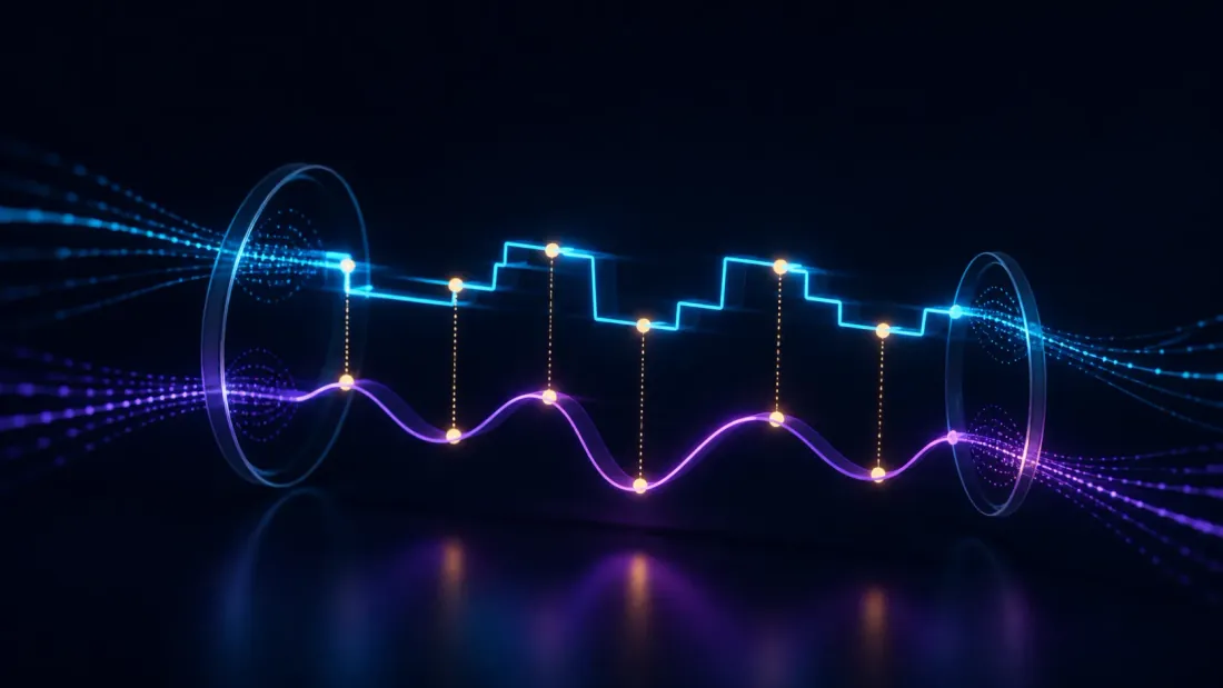
Esa propiedad tiene un atractivo obvio para los datos financieros, que llegan a intervalos aleatorios. Pero el argumento esconde una afirmación mucho más débil de lo que parece. Un GRU simple entregó una función de entrada adicional: desde la observación anterior, también "sabe" cuánto tiempo pasó. La verdadera pregunta no es si los modelos de tiempo continuo pueden asimilar datos irregulares. Se trata de si la dinámica continua aprendida entre observaciones extrae algo que una característica de tiempo delta no le brinda ya, a un costo de inferencia de diez a cien veces mayor.
Este artículo configura ese experimento, brinda la cadena de herramientas completa para ejecutarlo e informa lo que la comparación debería mostrar para justificar la maquinaria. El lado del argumento de la construcción de barras (que el momento del comercio en sí mismo transmite una señal) se establece con evidencia medida en 17 tipos de barras en [más allá de las barras de tiempo] (/en/blog/post/beyond-time-bars-candle-construction); Aquí la única consecuencia que importa es la del modelado: el solucionador evalúa el estado oculto en valores arbitrarios. , por lo que no se necesita interpolación ni relleno.
La afirmación bajo prueba

Tres hipótesis anidadas, cada una estrictamente más sólida que la anterior:
- H1 — Un ajuste ODE-RNN en un flujo comercial irregular de BTC supera a un ajuste GRU en el mismo flujo sin ninguna información de tiempo. Esto es casi seguro y casi inútil: el ODE-RNN simplemente tiene información de la que carece la línea base.
- H2 — El ODE-RNN supera al mismo GRU una vez que se proporciona el GRU como característica de entrada. Esta es la prueba honesta. Es la afirmación que generalmente se lee en la literatura sobre EDO neuronal, y es la que casi nunca se demuestra en los datos financieros.
- H3: la ventaja H2 sobrevive al presupuesto de latencia, es decir, se mantiene cuando ODE-RNN se implementa con un solucionador de pasos fijos lo suficientemente rápido para la inferencia en vivo en lugar de un solucionador adaptativo.
dopri5.
Protocolo de experimento
El mismo flujo de ticks, el mismo objetivo, el mismo presupuesto de ajuste para ambos brazos. No se requiere remuestreo en barras de 1 m: el remuestreo destruye la estructura exacta que se está probando.
| Configuración | |
|---|---|
| Datos | Impresiones comerciales de BTC, tiempos variables entre llegadas, no remuestreadas |
| Armas | ODE-RNN; gru + ; GRU sin función de tiempo |
| Objetivo | Lo mismo para todas las armas; especificado con el ajuste |
| Métricas | RMSE, probabilidad logarítmica retenida, reloj de pared por época, latencia de inferencia por paso |
| Barrido del solucionador | dopri5 (rtol 1e-5) vs Euler de paso fijo, igualados en precisión de entrenamiento |
| Dividir | Avance, solo fuera de muestra |
| Brazo | RMSE | Registro similar | s/época | Latencia/paso de inferencia |
|---|---|---|---|---|
| GRU (sin función de tiempo) | — | — | — | — |
| GRU + registro(dt) | — | — | — | — |
| ODE-RNN (dopri5) | — | — | — | — |
| ODE-RNN (Euler de paso fijo) | — | — | — | — |
Un resultado negativo en H2 es totalmente publicable y posiblemente sea el resultado más valioso: se aplica el mismo estándar en el resultado negativo honesto y Sharpe desinflado bajo múltiples pruebas.
Experimento secundario: CNF vs Student-t
Si la comparación ODE-RNN es demasiado costosa, el ancla empírica más barata es distribucional: ajuste un flujo de normalización continuo en los rendimientos diarios reales de BTC y compare su densidad ajustada con un ajuste t de Student y con la cola empírica, informando errores cuantiles de cola en los niveles del 1% y el 5%. Eso se conecta directamente con el trabajo de distribución ya medido en pronóstico de volatilidad GARCH y GARCH asimétrico.
El resto de este artículo son los antecedentes y la cadena de herramientas necesarias para ejecutar lo anterior.
Antecedentes: de ResNets a dinámicas continuas

Una red residual calcula . Reduzca el tamaño del paso y aumente el número de capas y se acercará a un límite continuo:
En lugar de Capas discretas con parámetros separados, una sola red. Especifica la tasa de cambio instantánea. La salida en el momento resuelve un problema de valor inicial:
Un solucionador de caja negra (Euler, Runge-Kutta, Dormand-Prince) calcula la integral numéricamente, eligiendo de forma adaptativa tamaños de paso a partir de estimaciones de error locales.
El método adjunto
La retropropagación a través de cada paso del solucionador almacena todos los estados intermedios, lo que cuesta memoria proporcional al recuento de pasos. Chen et al. en su lugar resuelve una EDO hacia atrás con memoria. Definir el estado adjunto , que satisface
y acumular el gradiente del parámetro a lo largo del paso hacia atrás:
El pase hacia atrás resuelve un sistema de computación aumentada , y simultáneamente, ejecutando el solucionador en reversa desde a .
La compensación: reconstruir al revés acumula error numérico, especialmente en dinámicas rígidas o caóticas. Los puntos de control son el término medio: tienda en algunos momentos intermedios, vuelva a calcular entre ellos. Los procesos de precios son semimartingalas continuas y moderadamente suaves, por lo que el adjunto generalmente se mantiene; La rigidez alrededor de los eventos de la microestructura puede obligar a solucionadores adaptativos o híbridos.
ODE-RNN: estado oculto continuo entre observaciones

ODE-RNN es la arquitectura que activa el experimento principal. Entre observaciones, el estado oculto evoluciona bajo la ODE:
cuando la observación llega a , se activa una actualización discreta:
Los superíndices denotan el estado justo antes y después de la observación. Entre observaciones, aprendió dinámica continua; en observaciones, nueva información.
El mecanismo que investigan las sondas de ablación con H2 es el siguiente: una brecha larga significa que el estado oculto ha evolucionado mucho bajo – decayendo hacia una línea de base, o divergiendo – y la forma de esa evolución se aprende en lugar de proporcionarse como un escalar. Lo que no se mide es exactamente si esa expresividad se amortiza con datos comerciales reales.
Ajustes naturales más allá de los ticks: carteras de activos múltiples donde cada activo tiene su propio cronograma de observación y el estado latente de los activos correlacionados sigue evolucionando mientras solo se observa uno; y señales impulsadas por eventos (noticias, resultados, publicaciones macroeconómicas) que llegan en momentos irregulares.
SDE neuronales: agregar componentes estocásticos

Las EDO neuronales son deterministas y no pueden representar el ruido en la trayectoria de un precio. El tratamiento clásico (movimiento browniano geométrico, deriva neutral al riesgo y las formas en que los supuestos de volatilidad constante fallan contra la sonrisa) se trata en Precios de opciones de Black-Scholes. Las SDE neuronales reemplazan la forma paramétrica con un término de difusión aprendido:
es la deriva, la difusión, un proceso Wiener, tanto y redes neuronales.
Arquitectura: red de deriva y red de difusión
- Red de deriva : trayectoria esperada: tendencia, reversión a la media, impulso. Entrenado para minimizar el error de predicción.
- Red de difusión : magnitud del ruido, aprendida en función del estado. Alto en regímenes volátiles, bajo en los tranquilos.
La división refleja las finanzas cuantitativas clásicas: la deriva es la dinámica neutral al riesgo (o medida P), la difusión es la superficie de volatilidad.
Entrenamiento de SDE neuronales
La integral estocástica no es clásicamente diferenciable. Tres enfoques:
- Gradientes de ruta: truco de reparametrización: muestrear rutas brownianas, diferenciarlas a través del solucionador que trata el ruido como una entrada fija.
- Coincidencia de puntuación: estimación y entrenar a través de objetivos de eliminación de ruido: la misma maquinaria utilizada como modelo generativo independiente en modelos de difusión para predicción criptográfica, aquí degradado a una opción de entrenamiento para el SDE.
- Coincidencia de distribución de dimensión finita: haga coincidir los marginales en los momentos de observación en lugar de las medidas de ruta completa.
Pathwise es el valor predeterminado práctico. torchsde implementa Euler-Maruyama, Milstein y estocástico Runge-Kutta con soporte autodiff.
Aprendiendo la superficie de volatilidad
Los modelos clásicos (Heston, SABR) imponen formas paramétricas al coeficiente de difusión. Un SDE neuronal aprende como función arbitraria:
Este es un aproximador universal para los procesos de difusión: cualquier proceso Ito con precisión arbitraria dada la capacidad suficiente.
EDO latentes para datos faltantes y asincrónicos

La EDO latente (Rubanova, Chen, Duvenaud, 2019) combina una EDO neuronal con una VAE: las series financieras son observaciones ruidosas de un proceso subyacente fluido, aprendido en un espacio latente de baja dimensión.
- Red de reconocimiento: una ODE-RNN que se ejecuta hacia atrás a través de observaciones para producir .
- Dinámica latente: .
- Decodificador: , evaluable en cualquier momento solicitado.
La pérdida es el ELBO estándar:
Estimación del estado de la cartera: a partir de escasas observaciones asincrónicas entre activos, infiere un estado latente continuo que captura la dinámica conjunta, esencialmente una versión aprendida y no lineal del filtro de Kalman.
Imputación de datos faltantes: las paradas y los intervalos de fin de semana obtienen una trayectoria latente interpolada suavemente; el decodificador produce caminos plausibles a través del espacio con incertidumbre del VAE posterior.
Fusión multifrecuencia: cierres diarios, VWAP intradiario y datos de ticks en un modelo sin una grilla horaria compartida.
Flujos de normalización continua para distribuciones de retorno
Los CNF utilizan una ODE neuronal para transformar una distribución base simple en un objetivo complejo. La transformación es , y la densidad logarítmica sigue el cambio instantáneo de variables:
Integre el estado y la densidad logarítmica hacia adelante desde Llegar y . La traza jacobiana se estima con el estimador estocástico de escalabilidad de Hutchinson.
Los rendimientos de las criptomonedas son leptocúrticos y están sesgados negativamente, medidos con datos reales en pronóstico de volatilidad de GARCH y GARCH asimétrico y el efecto de apalancamiento — y un CNF aprende esa forma en lugar de asumirla. Condicionar el flujo en variables de estado permite que la forma cambie con el régimen. Debido a que la densidad es exacta en lugar de aproximada, puede alimentar las métricas de cola calculadas en Monte Carlo y bootstrap backtests y la construcción de CVaR en el proceso de cartera HRP/CVaR; La estructura de la cola conjunta se maneja por separado en [modelos de cópula para riesgo conjunto] (/en/blog/post/copula-models-joint-risk-crypto).
Estimación de densidad condicional
El marco útil es un contraste directo entre tres enfoques publicados para el mismo problema. TFT le ofrece un conjunto fijo de cuantiles a partir de una capa de salida de cuantiles. Predicción conforme le ofrece intervalos calibrados con una garantía de cobertura. Un CNF condicional le proporciona una densidad exacta y diferenciable:
La diferenciabilidad es la propiedad distintiva: la densidad puede ubicarse dentro de un objetivo aguas abajo y propagarse hacia atrás, lo que ni los cuantiles fijos ni los intervalos conformes admiten. Aquí no se ha probado si la densidad exacta vale su costo frente a los cuantiles TFT en el mismo objetivo.
Comparación con alternativas discretas
| Propiedad | LSTM/GRU | Transformador | ODA neuronal | SDE neuronal |
|---|---|---|---|---|
| Manejo irregular del tiempo | Pobre (necesita relleno) | Codificación posicional | Nativo | Nativo |
| Memoria (entrenamiento) | adjunto | adjunto | ||
| Cuantificación de la incertidumbre | No (determinista) | No (determinista) | Vía conjuntos | Nativo |
| Interpolación entre observaciones | No | No | Sí | Sí |
| Densidad de tiempo continuo | No | No | Vía CNF | A través de medida de ruta |
| Costo computacional | Bajo | Moderado | Variable (solucionador) | Alto (solucionador SDE) |
La mitad LSTM versus atención de esta tabla se explica en detalle, con puntos de referencia, en el artículo de TFT; consulte las secciones "TFT vs LSTM vs Vanilla Transformer" y "Cuando LSTM aún gana". Las columnas que son nuevas aquí son las dos de la derecha, y las filas que deciden las preguntas H2/H3 son las dos últimas.
Implementación de Python con torchdiffeq
torchdiffeq proporciona solucionadores de ODE con retropropagación adjunta.
EDO neuronal básica para la dinámica de precios
import torch
import torch.nn as nn
from torchdiffeq import odeint_adjoint as odeint

class PriceDynamics(nn.Module):
    """Neural network defining dh/dt = f(h, t)."""

    def __init__(self, hidden_dim: int = 64):
        super().__init__()
        self.net = nn.Sequential(
            nn.Linear(hidden_dim, 128),
            nn.Tanh(),
            nn.Linear(128, 128),
            nn.Tanh(),
            nn.Linear(128, hidden_dim),
        )

    def forward(self, t, h):
        return self.net(h)


class NeuralODEPredictor(nn.Module):
    """
    Encode observed features -> latent state,
    evolve via Neural ODE,
    decode to price prediction.
    """

    def __init__(self, input_dim: int, hidden_dim: int = 64):
        super().__init__()
        self.encoder = nn.Linear(input_dim, hidden_dim)
        self.dynamics = PriceDynamics(hidden_dim)
        self.decoder = nn.Linear(hidden_dim, 1)

    def forward(self, x0, eval_times):
        """
        x0:         (batch, input_dim) features at t=0
        eval_times: (T,) times at which to evaluate the ODE
        Returns:    (T, batch, 1) predictions
        """
        h0 = self.encoder(x0)                          # (batch, hidden_dim)
        h_traj = odeint(self.dynamics, h0, eval_times,
                        method='dopri5', rtol=1e-5, atol=1e-7)
        return self.decoder(h_traj)
ODE-RNN para datos de ticks irregulares
Este es el brazo experimental. La base que debe superar es nn.GRUCell en la misma corriente con log(t_next - t_prev) concatenado a x.
class ODERNNCell(nn.Module):
    """Single step: ODE-evolve, then RNN-update."""

    def __init__(self, input_dim: int, hidden_dim: int = 64):
        super().__init__()
        self.dynamics = PriceDynamics(hidden_dim)
        self.gru_cell = nn.GRUCell(input_dim, hidden_dim)

    def forward(self, h, x, t_prev, t_next):
        times = torch.tensor([t_prev, t_next], dtype=torch.float32)
        h_evolved = odeint(self.dynamics, h, times,
                           method='dopri5')[-1]  # state at t_next
        h_updated = self.gru_cell(x, h_evolved)
        return h_updated


class ODERNN(nn.Module):
    """Process irregularly-sampled sequence."""

    def __init__(self, input_dim: int, hidden_dim: int = 64):
        super().__init__()
        self.cell = ODERNNCell(input_dim, hidden_dim)
        self.decoder = nn.Linear(hidden_dim, 1)
        self.hidden_dim = hidden_dim

    def forward(self, observations, times):
        """
        observations: list of (batch, input_dim) tensors
        times:        list of floats, observation timestamps
        """
        batch_size = observations[0].shape[0]
        h = torch.zeros(batch_size, self.hidden_dim)

        outputs = []
        for i in range(len(observations)):
            t_prev = 0.0 if i == 0 else times[i - 1]
            h = self.cell(h, observations[i], t_prev, times[i])
            outputs.append(self.decoder(h))

        return torch.stack(outputs)  # (seq_len, batch, 1)
Bucle de entrenamiento
def train_neural_ode(model, train_loader, epochs=100, lr=1e-3):
    optimizer = torch.optim.Adam(model.parameters(), lr=lr)
    scheduler = torch.optim.lr_scheduler.CosineAnnealingLR(
        optimizer, T_max=epochs
    )

    for epoch in range(epochs):
        epoch_loss = 0.0
        for batch in train_loader:
            features, times, targets = batch
            optimizer.zero_grad()

            predictions = model(features, times)
            loss = torch.nn.functional.mse_loss(predictions, targets)

            loss.backward()
            torch.nn.utils.clip_grad_norm_(model.parameters(), max_norm=1.0)
            optimizer.step()

            epoch_loss += loss.item()

        scheduler.step()

        if (epoch + 1) % 10 == 0:
            avg_loss = epoch_loss / len(train_loader)
            print(f"Epoch {epoch+1}/{epochs}, Loss: {avg_loss:.6f}")
Flujo de normalización continua para distribuciones de retorno
from torchdiffeq import odeint

class CNFDynamics(nn.Module):
    """Dynamics for continuous normalizing flow."""

    def __init__(self, dim: int = 1, hidden_dim: int = 64):
        super().__init__()
        self.net = nn.Sequential(
            nn.Linear(dim + 1, hidden_dim),  # +1 for time
            nn.Tanh(),
            nn.Linear(hidden_dim, hidden_dim),
            nn.Tanh(),
            nn.Linear(hidden_dim, dim),
        )
        self.dim = dim

    def forward(self, t, state):
        z = state[..., :self.dim]
        t_expand = t.expand(z.shape[0], 1)
        zt = torch.cat([z, t_expand], dim=-1)
        dz = self.net(zt)

        e = torch.randn_like(z)
        e_dz = torch.autograd.grad(
            dz, z, e, create_graph=True
        )[0]
        trace_jac = (e_dz * e).sum(dim=-1, keepdim=True)

        return torch.cat([dz, -trace_jac], dim=-1)


class ReturnDistributionCNF(nn.Module):
    """Model return distributions with continuous normalizing flows."""

    def __init__(self, dim: int = 1):
        super().__init__()
        self.dynamics = CNFDynamics(dim)
        self.dim = dim

    def log_prob(self, x):
        """Compute log probability of observed returns."""
        log_p0 = torch.zeros(x.shape[0], 1)
        state0 = torch.cat([x, log_p0], dim=-1)
        state0.requires_grad_(True)

        times = torch.tensor([1.0, 0.0])  # backward
        state_T = odeint(self.dynamics, state0, times,
                         method='dopri5')[-1]

        z_T = state_T[..., :self.dim]
        delta_log_p = state_T[..., self.dim:]

        log_p_base = -0.5 * (z_T ** 2 + torch.log(
            torch.tensor(2 * torch.pi)
        )).sum(dim=-1, keepdim=True)

        return log_p_base + delta_log_p

    def sample(self, n_samples: int):
        """Generate samples from learned distribution."""
        z0 = torch.randn(n_samples, self.dim)
        log_p0 = torch.zeros(n_samples, 1)
        state0 = torch.cat([z0, log_p0], dim=-1)

        times = torch.tensor([0.0, 1.0])  # forward
        state_T = odeint(self.dynamics, state0, times,
                         method='dopri5')[-1]

        return state_T[..., :self.dim]
Notas prácticas

Estas son las cosas que te molestarán mientras realizas el experimento anterior.
Elección y velocidad del solucionador
dopri5 ofrece garantías de precisión pero un costo de cómputo variable, razón por la cual H3 es una hipótesis separada de H2: una ventaja que solo existe bajo un solucionador adaptativo puede no sobrevivir a un presupuesto de latencia activa. Los solucionadores de pasos fijos (Euler, RK4) brindan una latencia predecible a costa de la precisión. Compromiso práctico: entrenar con dopri5, implemente con un solucionador de pasos fijos calibrado para que coincida con la salida del solucionador adaptativo en datos representativos y mida la brecha en lugar de asumir que es pequeña.
odeint(f, h0, t, method='dopri5', rtol=1e-6, atol=1e-8)

odeint(f, h0, t, method='euler', options={'step_size': 0.1})
Para problemas rígidos cerca de saltos discontinuos, method='implicit_adams' o method='scipy_solver'.
Estabilidad numérica
si genera valores grandes, el estado diverge. Mitigaciones:
- Normalización espectral en capas de para controlar la constante de Lipschitz.
- Recorte de gradiente durante el entrenamiento (como se muestra en el bucle de entrenamiento anterior).
- Normalización de tiempo: escalar marcas de tiempo a .
- Regularización sobre norma dinámica: agregar a la perdida.
Intervalo de integración
Para datos que abarcan meses, no integre desde a minutos:
t_normalized = (timestamps - timestamps[0]) / (timestamps[-1] - timestamps[0])
Esto mantiene al solucionador en un régimen numéricamente amigable y hace que la dinámica aprendida sea invariante en escala. También es importante para la comparación: un ODE-RNN no normalizado puede perder respecto a la línea base de GRU por razones puramente numéricas, lo que sería un artefacto de medición en lugar de un hallazgo.
Manejo de múltiples escalas de tiempo
Los mercados tienen dinámicas a escalas de microsegundos, segundos, minutos y diarias a la vez, y una sola EDO neuronal puede tener dificultades para contenerlas todas. Opciones: apilar múltiples bloques ODE en diferentes escalas de tiempo; ampliar la dimensión oculta para capacidad tanto rápida como lenta; o ejecute ODE neuronales separadas por banda de frecuencia y salidas de fusibles. (Esta es una pregunta sobre la capacidad del modelo, distinta de la pregunta sobre la fidelidad del backtest en desglose de la resolución adaptativa.)
Direcciones de investigación abiertas

Neural Jump SDE: agregue un componente de salto aprendido para dislocaciones repentinas (caídas repentinas, sorpresas en las ganancias):
dónde es una medida aleatoria de Poisson compensada y un núcleo de salto aprendido.
Ecuaciones diferenciales controladas neuronalmente (CDE neuronales): reemplace el proceso de Wiener con una señal de conducción general, permitiendo que los flujos de datos observados impulsen la dinámica. Natural para el flujo de órdenes, donde el flujo de operaciones y cotizaciones impulsa el estado latente del mercado.
Simulación de mercado diferenciable: use un SDE neuronal como modelo generativo dentro de un simulador diferenciable y entrene estrategias de un extremo a otro mediante la retropropagación a través de él a través del adjunto. La estrategia y el modelo de mercado coevolucionan.
ODE neuronales basadas en la física: los PINN incorporan una ecuación diferencial residual en la pérdida; la técnica en sí se presenta en el artículo de Navier-Stokes. La aplicación financiera es imponer condiciones de no arbitraje, paridad de compra y martingala como términos de penalización o restricciones estrictas a la dinámica aprendida.
Conclusión

El marco de tiempo continuo es estructuralmente correcto: los mercados son procesos continuos observados en momentos discretos e irregulares, y los modelos deberían respetar eso. La cadena de herramientas está madura. torchdiffeq, torchsde, PyTorch simple para el resto, y los costos conocidos son la velocidad del solucionador y la estabilidad numérica durante largos intervalos de integración.
Lo que no está establecido es la parte que decide si algo de esto pertenece a una pila de producción. La corrección estructural no es evidencia de ventaja predictiva, y la ventaja específica reivindicada para la dinámica continua sobre una La característica no se ha medido aquí con datos comerciales reales. Hasta que se complete la tabla H2 anterior, trate todo lo que se encuentra debajo como una hipótesis bien especificada con una implementación funcional adjunta, no como un resultado.
Referencias
- Chen, RTQ, Rubanova, Y., Bettencourt, J., Duvenaud, D. (2018). Ecuaciones diferenciales neuronales ordinarias. NeurIPS 2018. arXiv:1806.07366
- Rubanova, Y., Chen, RTQ, Duvenaud, D. (2019). EDO latentes para series temporales muestreadas irregularmente. NeurIPS 2019. arXiv:1907.03907
- Jia, J., Benson, AR. (2019). Ecuaciones diferenciales estocásticas de salto neuronal. NeuroIPS 2019.
- Kidger, P., Morrill, J., Foster, J., Lyons, T. (2020). Ecuaciones diferenciales controladas neuronalmente para series temporales irregulares. NeuroIPS 2020.
- Hasan, A., Pereira, JM, Farsiu, S., Carin, L. (2021). Modelos de ecuaciones diferenciales estocásticas de redes neuronales con aplicaciones a la previsión de datos financieros. arXiv:2111.13164
- antorchadiffeq: github.com/rtqichen/torchdiffeq
- Tutoriales de aprendizaje profundo de UvA: EDO neuronales: uvadlc-notebooks.readthedocs.io
Authors
Trading-systems engineer
Trading-systems engineer building bots since 2017: cross-exchange arbitrage (connected up to 30 venues), cointegration-based pairs arbitrage across spot and futures, scalping, news and sentiment-driven strategies, trend algorithms, and portfolio management and balancing algorithms. Also builds sub-millisecond order execution, big-data warehouses, backtesting engines, AI agents, and trading interfaces (incl. open-source profitmaker.cc). Stack: JS/TS, Python, Rust/Zig/Go, DevOps, backend, frontend, architecture.
Read More

Hamiltonian Neural Networks: Does a Financial System Conserve Anything?

Trade Classification When You Have No Side Flag: Tick, Quote, Lee-Ready, BVC