Fourier neurale operator voor op PDE gebaseerde financiële modellering
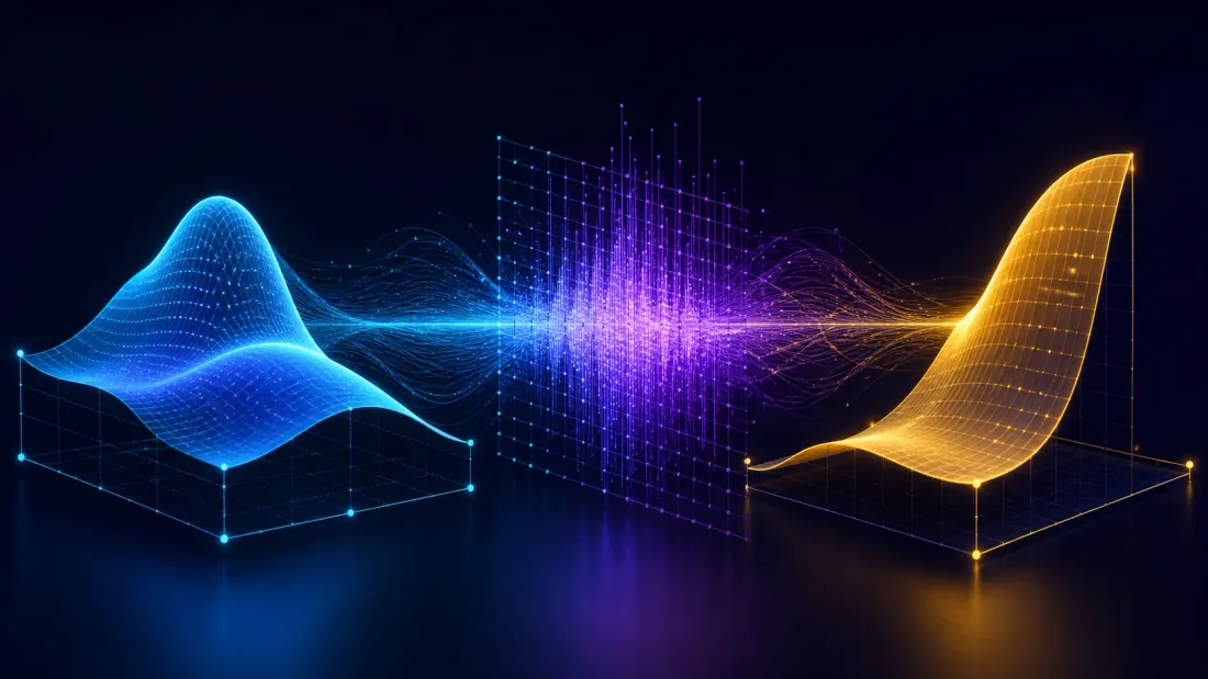
Elk neuraal netwerk op deze blog tot nu toe heeft ongeveer een functie benaderd: features erin, een getal eruit. De Fourier neurale operator benadert een operator: een kaart tussen oneindig-dimensionale functieruimten, waarbij de input een heel volatiliteitsoppervlak is en de output een heel prijsoppervlak. Dat is een ander object, het heeft een andere machinerie nodig, en die machinerie is het punt van dit artikel: een leerbare kernel met complexe waarden toegepast op de laagste Fourier-modi, geëvalueerd via een FFT-retour in .
Optieprijzen is waar dit in de financiële sector terechtkomt. Black-Scholes, Heston, lokale volatiliteit – alle PDE’s, vandaag allemaal opgelost met één parameter tegelijk. Een operator leert de hele parameterfamilie in één keer kennen, en de resulterende voorwaartse doorgang is een enkele batch-GPU-kernel in plaats van een tijdmarsende lus.
Dat is de belofte. De eerlijke versie van dit artikel scheidt de mechanismen, die solide en reproduceerbaar zijn uit de onderstaande code, van de prestatieclaims, die in de FNO-literatuur worden gerapporteerd tegen basislijnen die niemand in deze serie zonder onderzoek zou accepteren. De mechanica komt op de eerste plaats; de meetagenda komt aan het einde en is gemarkeerd als niet uitgevoerd.
Van functiebenadering tot leren van operators
Klassieke neurale netwerken benaderen functies: gegeven een input , produceren ze een output . Dit is krachtig, maar fundamenteel beperkt wanneer de objecten van belang zelf functies zijn. Bij het oplossen van financiële PDE's is de invoer niet een enkel getal; het is een functie die initiële/randvoorwaarden, een volatiliteitsoppervlak of een termstructuur beschrijft. De output is een andere functie: het prijsoppervlak stijgt ruimte.
Operator learning tilt het probleem naar oneindig-dimensionale ruimtes. In plaats van te leren , leren we een operator:
waar En zijn Banachruimten van functies. Voor optieprijzen, zou de ruimte van volatiliteitsoppervlakken kunnen zijn En de ruimte van overeenkomstige prijsoppervlakken .
Twee architecturen domineren het leerlandschap van operators:
-
DeepONet (Lu et al., 2021): gebruikt een vestigingsnetwerk om de invoerfunctie te coderen en een trunknetwerk om de vraaglocatie te coderen. De output is hun inproduct. Gebaseerd op de universele benaderingsstelling voor operatoren van Chen en Chen (1995).
-
Fourier neurale operator (Li et al., 2021): parameteriseert de integrale kernel in de Fourier-ruimte, met behulp van de FFT voor efficiënte mondiale convolutie. Resolutie-invariant door constructie.
Beide zijn universele benaderingen voor continue operatoren, maar FNO heeft een structureel voordeel voor PDE-problemen: de spectrale bias weerspiegelt op natuurlijke wijze de soepele, globale structuur van PDE-oplossingen. Het heeft ook een structureel nadeel voor met name de uitbetaling van opties, waar we nog op terug zullen komen: een ingekorte Fourier-basis en een knik in de staking zijn geen natuurlijke bondgenoten.
FNO-architectuur in detail
De Fourier neurale operator, geïntroduceerd door Li et al. op ICLR 2021, bouwt voort op een eenvoudige maar krachtige observatie: de Groene functie (integrale kern) van veel PDE's heeft een compacte representatie in de Fourier-ruimte. In plaats van een kernel in de fysieke ruimte te leren – wat vereist parameters voor rasterpunten — FNO leert het in de frequentieruimte met alleen de laagste modi, waardoor de complexiteit wordt verminderd via de FFT.
De iteratieve architectuur
Een FNO bestaat uit:
-
Hijslaag : Een puntsgewijze lineaire kaart die de invoer van de oorspronkelijke kanaaldimensie projecteert naar een hoger-dimensionale latente representatie: .
-
Fourier-lagen (herhaald keer): Elke laag is van toepassing:
waar is een lokale lineaire transformatie (puntsgewijs convolutie) en is een mondiale integrale operator geïmplementeerd via de FFT:
Hier geeft de FFT aan, is een leerbare gewichtstensor met complexe waarde, toegepast op de laagste Fourier-modi, en is een puntsgewijze niet-lineaire activering (typisch GELU).
- Projectielaag : Brengt de latente representatie terug naar de uitvoerdimensie: .
Waarom Fourierruimte?
De spectrale convolutie is een vermenigvuldiging in het frequentiedomein, wat equivalent is aan een globale convolutie in de fysieke ruimte – maar dan berekend in plaats van . Dit is niet alleen een efficiëntietruc. PDE-oplossingen zijn doorgaans soepel en worden gedomineerd door laagfrequente componenten. Door af te korten naar In de modi fungeert FNO als een leerbaar laagdoorlaatfilter dat de oplossing op natuurlijke wijze regulariseert en hoogfrequente artefacten vermijdt.
Cruciaal is dat FNO wordt beweerd discretisatie-invariant te zijn: eenmaal getraind op een raster van grootte , kan het op elke resolutie worden geëvalueerd door simpelweg de FFT-grootte aan te passen en de spectrale gewichten op nul te zetten of in te korten. Deze zero-shot superresolutie-eigenschap is uniek onder neurale PDE-oplossers – en het is de eerste claim in dit artikel die een meting verdient in plaats van een citaat. Zie onderstaande meetagenda.
De PDE waarvoor we de operator leren
De Black-Scholes PDE – afgeleid, term voor term ontleed, en gegeven met zijn call/put-oplossing in gesloten vorm in [The Black-Scholes Formula] (/nl/blog/post/black-scholes-options-pricing) – is het doel van de operator:
Alles wat volgt beschouwt het als een zwarte doos met een bekend antwoord. Dat bekende antwoord is precies waarom het de juiste testcase is: een operator die getraind is in output met eindige verschillen kan worden gescoord tegen norm.cdf exacte prijzen, wat bijna geen enkele FNO-benchmark in de literatuur kan doen.
FNO-formulering
We herschrijven het probleem als operator learning. Definieer:
- Invoerfunctie : codeert de PDE-parameters. Dit kan het vluchtigheidsoppervlak omvatten , de uitbetalingsfunctie en de risicovrije rente als kanalen die op de rooster.
- Uitvoerfunctie : het optieprijsoppervlak.
De FNO leert uit een dataset van paren gegenereerd door een traditionele oplosser. Na de training is de gevolgtrekking voor elke nieuwe parameterconfiguratie een enkele voorwaartse doorgang.
Generatie van trainingsgegevens
import numpy as np
from scipy.stats import norm

def black_scholes_fd(sigma, r, K, T, S_max=300, N_S=256, N_t=256):
    """Solve Black-Scholes PDE via explicit finite differences.

    NOTE: this is an interpreted double loop — the *worst* CPU baseline,
    exactly the kind called out in /en/blog/post/when-gpu-pays-off-sweep-roofline.
    It is fine for generating training data offline. It is NOT the baseline
    any speedup claim should be measured against; vectorize the inner loop
    over i (or use scipy sparse + implicit stepping) before timing anything.
    """
    dS = S_max / N_S
    dt = T / N_t
    S = np.linspace(0, S_max, N_S + 1)

    V = np.maximum(S - K, 0).astype(np.float64)

    for j in range(N_t):
        V_new = V.copy()
        for i in range(1, N_S):
            delta = (V[i+1] - V[i-1]) / (2 * dS)
            gamma = (V[i+1] - 2*V[i] + V[i-1]) / (dS**2)
            V_new[i] = V[i] + dt * (
                0.5 * sigma**2 * S[i]**2 * gamma
                + r * S[i] * delta
                - r * V[i]
            )
        V_new[0] = 0
        V_new[N_S] = S_max - K * np.exp(-r * (T - (j+1)*dt))
        V = V_new

    return S, V
Voor training testen we duizenden parameterconfiguraties, variërend , , , - en elk probleem oplossen met de eindige-verschilmethode. De resulterende dataset van input-output-paren is waar de FNO van leert.
Opschalen: het stochastische volatiliteitsmodel van Heston
Constante volatiliteit is een bekende en onjuiste aanname, en waarom deze faalt – de glimlach, de dikke staarten – is het onderwerp van de sectie ‘Harsh Reality’ van The Black-Scholes Formula. Heston lost dit op door van variantie een tweede toestandsvariabele te maken:
met . De bijbehorende PDE voor de optieprijs is tweedimensionaal in de ruimte:
Dit is waar het leren van operators zijn geld verdient, en het argument is eerder structureel dan empirisch. Eindige-verschilschema's op a rasterschaal als , de afgeleide term bemoeilijkt de discretisatie en elke nieuwe parameterset betaalt opnieuw de volledige kosten. Een operator betaalt dit eenmalig tijdens de training. De ruimtelijke 2D-structuur van de Heston PDE komt ook rechtstreeks overeen met de 2D FFT in de Fourier-lagen, dus de onderstaande architectuur generaliseert met een dimensieverandering in plaats van een herontwerp.
FNO voor optieprijzen: PyTorch-implementatie
Hieronder vindt u een complete, op zichzelf staande FNO-implementatie voor het leren van de Black-Scholes-operator. De architectuur volgt Li et al. (2021) met aanpassingen voor de financiële setting.
import torch
import torch.nn as nn
import torch.nn.functional as F
from torch.fft import rfft, irfft

class SpectralConv1d(nn.Module):
    """1D Fourier layer: spectral convolution via FFT."""

    def __init__(self, in_channels: int, out_channels: int, modes: int):
        super().__init__()
        self.in_channels = in_channels
        self.out_channels = out_channels
        self.modes = modes  # Number of Fourier modes to keep

        scale = 1.0 / (in_channels * out_channels)
        self.weights = nn.Parameter(
            scale * torch.randn(in_channels, out_channels, modes, dtype=torch.cfloat)
        )

    def forward(self, x: torch.Tensor) -> torch.Tensor:
        batch_size = x.shape[0]

        x_ft = rfft(x, dim=-1)

        out_ft = torch.zeros(
            batch_size, self.out_channels, x_ft.size(-1),
            dtype=torch.cfloat, device=x.device
        )
        out_ft[:, :, :self.modes] = torch.einsum(
            "bix,iox->box", x_ft[:, :, :self.modes], self.weights
        )

        return irfft(out_ft, n=x.size(-1), dim=-1)


class FNOBlock(nn.Module):
    """Single Fourier Neural Operator block."""

    def __init__(self, channels: int, modes: int):
        super().__init__()
        self.spectral_conv = SpectralConv1d(channels, channels, modes)
        self.pointwise = nn.Conv1d(channels, channels, kernel_size=1)
        self.norm = nn.InstanceNorm1d(channels)

    def forward(self, x: torch.Tensor) -> torch.Tensor:
        return F.gelu(self.norm(self.spectral_conv(x) + self.pointwise(x)))


class FNO1d(nn.Module):
    """
    Fourier Neural Operator for 1D PDE problems.

    Learns the mapping: PDE parameters -> solution function
    """

    def __init__(
        self,
        in_channels: int = 3,    # e.g., sigma(S), payoff(S), grid(S)
        out_channels: int = 1,   # V(S)
        hidden_channels: int = 64,
        modes: int = 32,
        num_layers: int = 4,
    ):
        super().__init__()
        self.lift = nn.Linear(in_channels, hidden_channels)
        self.blocks = nn.ModuleList(
            [FNOBlock(hidden_channels, modes) for _ in range(num_layers)]
        )
        self.proj = nn.Sequential(
            nn.Linear(hidden_channels, 128),
            nn.GELU(),
            nn.Linear(128, out_channels),
        )

    def forward(self, x: torch.Tensor) -> torch.Tensor:
        x = self.lift(x)                    # -> (batch, spatial, hidden)
        x = x.permute(0, 2, 1)              # -> (batch, hidden, spatial)

        for block in self.blocks:
            x = block(x)

        x = x.permute(0, 2, 1)              # -> (batch, spatial, hidden)
        return self.proj(x)                  # -> (batch, spatial, out_channels)
Trainingslus
import torch.optim as optim
from torch.utils.data import DataLoader, TensorDataset

def train_fno_black_scholes():
    device = torch.device("cuda" if torch.cuda.is_available() else "cpu")

    N_samples = 5000
    N_S = 256
    S_max = 300.0
    S_grid = np.linspace(0, S_max, N_S + 1)

    inputs, targets = [], []
    for _ in range(N_samples):
        sigma = np.random.uniform(0.05, 0.80)
        r = np.random.uniform(0.01, 0.10)
        K = np.random.uniform(50, 150)
        T = np.random.uniform(0.1, 2.0)

        _, V = black_scholes_fd(sigma, r, K, T, S_max=S_max, N_S=N_S)

        sigma_field = np.full(N_S + 1, sigma)
        payoff = np.maximum(S_grid - K, 0)
        grid_norm = S_grid / S_max

        inp = np.stack([sigma_field, payoff, grid_norm], axis=-1)
        inputs.append(inp)
        targets.append(V[:, None])

    X = torch.tensor(np.array(inputs), dtype=torch.float32)
    Y = torch.tensor(np.array(targets), dtype=torch.float32)

    dataset = TensorDataset(X, Y)
    loader = DataLoader(dataset, batch_size=64, shuffle=True)

    model = FNO1d(in_channels=3, out_channels=1, hidden_channels=64, modes=32).to(device)
    optimizer = optim.AdamW(model.parameters(), lr=1e-3, weight_decay=1e-4)
    scheduler = optim.lr_scheduler.CosineAnnealingLR(optimizer, T_max=200)

    for epoch in range(200):
        model.train()
        total_loss = 0.0
        for batch_x, batch_y in loader:
            batch_x, batch_y = batch_x.to(device), batch_y.to(device)

            pred = model(batch_x)
            loss = torch.mean(
                torch.norm(pred - batch_y, dim=1)
                / torch.norm(batch_y, dim=1).clamp(min=1e-8)
            )

            optimizer.zero_grad()
            loss.backward()
            optimizer.step()
            total_loss += loss.item()

        scheduler.step()
        if (epoch + 1) % 20 == 0:
            avg = total_loss / len(loader)
            print(f"Epoch {epoch+1:3d} | Relative L2 Loss: {avg:.6f}")

    return model
Gevolgtrekking: realtime prijzen
@torch.no_grad()
def price_option(model, sigma, K, S_grid, device="cuda"):
    """
    Price a European call for given sigma and strike.
    Returns prices for all S in S_grid — single forward pass.
    """
    S_max = S_grid[-1]
    payoff = np.maximum(S_grid - K, 0)
    grid_norm = S_grid / S_max
    sigma_field = np.full_like(S_grid, sigma)

    inp = np.stack([sigma_field, payoff, grid_norm], axis=-1)
    x = torch.tensor(inp, dtype=torch.float32).unsqueeze(0).to(device)

    pred = model(x)
    return pred.squeeze().cpu().numpy()
FNO versus PINN's: een praktische vergelijking
Physics-Informed Neural Networks en Fourier Neural Operators vertegenwoordigen fundamenteel verschillende filosofieën voor het oplossen van PDE's met neurale netwerken. Het begrijpen van hun afwegingen is de praktische reden om überhaupt aandacht te besteden aan het leren van operators.
PINN's: optimalisatie per exemplaar
PINN's plaatsen het PDE-residu direct in het verlies - [Het Navier-Stokes-probleem] (/nl/blog/post/navier-stokes-problem) behandelt het mechanisme, het autodiff physics_loss implementatie, en het DeepMind singulariteitszoekresultaat. De enige eigenschap die hier van belang is, is structureel: per parameterset wordt een PINN getraind. Wijziging , , of en je optimaliseert opnieuw vanaf nul.
Sterke punten: Geen gelabelde gegevens vereist. Dwingt direct de PDE-structuur af. Werkt voor elke PDE die u kunt opschrijven.
Zwakke punten: Moet opnieuw worden getraind voor elke nieuwe parameterset . Training omvat het balanceren van meerdere verliestermen (PDE-residu, randvoorwaarden, initiële voorwaarden), wat vaak leidt tot optimalisatiepathologieën. Convergentie kan langzaam verlopen: doorgaans 10.000 tot 100.000 gradiëntstappen per probleeminstantie. Mislukt op chaotische systemen op meerdere schaal waarbij het verlieslandschap zeer niet-convex wordt.
FNO: Geamortiseerde Operator Learning
FNO leert de oplossingsoperator uit data. Het vereist een trainingsdataset die is gegenereerd door een klassieke oplosser, maar zodra deze is getraind, generaliseert deze over de gehele parameterruimte.
Sterke punten: gevolgtrekkingen van minder dan een milliseconde in de gepubliceerde benchmarks. Generaliseert naar onzichtbare parameters zonder opnieuw te trainen. Resolutie-invariant: train met een lage resolutie, evalueer met een hoge resolutie. Verwerkt op natuurlijke wijze soepele PDE-oplossingen via spectrale bias.
Zwakke punten: Vereist trainingsgegevens van een klassieke oplosser (kip-en-ei-probleem voor echt nieuwe PDE's). De benaderingsfout is begrensd maar niet nul. Minder interpreteerbaar dan PDE-beperkte benaderingen. En de spectrale bias die helpt bij soepele oplossingen is een risico bij een knik in de uitbetaling.
Vergelijking van hoofd tot hoofd
De onderstaande tabel is in de literatuur gerapporteerd, hier niet gemeten – vooral de nauwkeurigheids- en versnellingsrijen zijn afkomstig van Li et al. (2021) en vervolgwerk op het gebied van vloeiende benchmarks, niet van optieprijzen op onze hardware. Lees de structurele rijen (benodigde gegevens, generalisatie, resolutie-invariantie) als de betrouwbare.
| Criterium | PINN | FNO |
|---|---|---|
| Trainingsgegevens nodig | Geen (zonder toezicht) | Door de oplosser gegenereerde paren |
| Inferentiekosten | Volledige omscholing per exemplaar | Enkele voorwaartse pas |
| Generalisatie | Enkele parameterset | Gehele parameterfamilie |
| Resolutie-invariantie | Nee | Beweerde ja — zie agenda hieronder |
| PDE's op meerdere schaal | Mislukt vaak | Robuust gerapporteerd |
| Nauwkeurigheid (relatief , literatuur) | naar | naar |
De hybride: op natuurkunde geïnformeerde neurale operators (PINO)
PINO (Li et al., 2024) combineert beide benaderingen. Het maakt gebruik van de FNO-architectuur, maar vergroot het datagestuurde verlies met een PDE-restterm:
De ontleding is het nuttige deel. verankert de operator aan de uitvoer van de oplosser, waar u deze ook heeft; beperkt het overal waar u dat niet doet, inclusief gebieden in de parameterruimte die u nooit hebt bemonsterd. Voor de prijsstelling van opties is die tweede termijn aantrekkelijk om een reden die specifiek is voor de financiering: het PDE-residu is een harde beperking die u ook tijdens de conclusie kunt evalueren als een zelfcontrole, wat de basis vormt van de onderstaande fallback voor residuele monitoring.
Praktische overwegingen voor productie-implementatie
De generieke helft hiervan – latentiebudgetten voor gevolgtrekkingen, het opbouwen van de datapijplijn, monitoring op drift, periodieke herscholing – is al gedekt voor een neuraal model in een handelssysteem in de productiesectie van DeepLOB: Deep Learning on Limit Order Books, en is ongewijzigd van toepassing. Wat volgt is alleen wat specifiek is voor een operator.
Datapijplijn: bemonstering van de parameterruimte
Het genereren van trainingsgegevens is het grootste knelpunt, en in tegenstelling tot een marktgegevensmodel kiest u uw eigen distributie – wat betekent dat u fouten kunt maken op een manier die onzichtbaar is in het verlies. Voor de Black-Scholes-operator met 4 parameters zijn 5.000–10.000 monsters voldoende. Voor Heston met 5 parameters plus een ruimtelijk 2D-domein zijn 20.000–50.000 monsters typisch. Gebruik adaptieve bemonstering: concentreer monsters in parametergebieden waar de oplossing snel varieert – bijna-the-money, korte looptijden, hoge volatiliteit – omdat uniforme bemonstering van de box het grootste deel van zijn budget besteedt aan deep-ITM- en deep-OTM-regio’s waar de operator bijna lineair is en goed leert van zeer weinig voorbeelden.
Architectuurafstemming
- ** Modi ** (): Begin met waar is de ruimtelijke rastergrootte. Voor , gebruik de modi 32–64. Te weinig modi verliezen details in de buurt van stakingsgrenzen; te veel mensen die te veel lawaai maken.
- Lagen: 4 Fourier-lagen zijn standaard. Diepere netwerken (6–8) helpen bij 2D-problemen zoals Heston, maar vergroten het geheugen.
- Verborgen kanalen: 64 voor 1D Black-Scholes, 128 voor 2D Heston. Schaal mee met de complexiteit van het probleem.
Precisie: de fp32-vraag
SpectralConv1d wijst toe torch.cfloat – complex met één precisie – en elke FFT-retour verloopt met die precisie. Deze blog heeft al gezien hoe een financiële pijplijn van fp32 stille rotzooi retourneerde in The GPU Precision Trap, waar een wiskundig correcte prefix-sum-formulering catastrofaal verloren ging bij fp32-grootheden. De analoge vraag hier is direct: op met prijzen tot op de cent, geldt een spectrale retourvlucht van fp32 absoluut, of eet de gemiddelde groei van de FFT de laatste significante cijfers op?
Foutcontrole
Voor de prijsbepaling van productieopties heeft u foutgrenzen nodig die u kunt verdedigen.
- Gekalibreerde onzekerheid: een standaarddeviatie van een ensemble is geen een dekkingsgarantie, en deze blog beschikt over de apparatuur om dit op de juiste manier te doen – conformeel opgesplitst over een vaststaand parameterraster, met ACI/DtACI voor het niet-uitwisselbare geval, in Conformele voorspelling voor risicobewuste positiebepaling. De FNO in split-conformal wikkelen over de grid geeft distributievrije intervallen op de prijs.
- Residuele monitoring: Bereken het PDE-residu van de FNO-voorspelling als een post-hoccontrole. Als , val terug op een klassieke oplosser. Dit is gratis bij gevolgtrekking: het residu is een stencil met eindige verschillen op een array die je al hebt.
- Actief leren: Stuur invoer met hoge onzekerheid door naar de klassieke oplosser, voeg de resultaten toe aan de trainingsset en train periodiek opnieuw. De conforme intervalbreedte uit (1) is het natuurlijke routeringssignaal.
De Meetagenda
Dit is het deel dat beslist of de bovenstaande architectuur de moeite waard is om te implementeren, en er is nog niets klaar. Het wordt hier vermeld in plaats van begraven, omdat het alternatief – het beweren van een versnelling van de krantenkoppen – precies het register is dat deze blog moet vermijden.
1. Snelheid is een curve, geen getal. When the GPU Pays Off bepaalt de vorm: , stijgend van door overhead gedomineerd bij naar een computergebonden plateau, en het toont een kop van 167x die uiteenvalt in 27x algoritme maal 6,2x hardware. De FNO-meting moet dat sjabloon volgen: wandklok de voorwaartse pas op en rapporteer de hele curve. Cruciaal is dat de basislijn een gevectoriseerde, multi-core eindige-verschiloplosser moet zijn – de black_scholes_fd hierboven is een geïnterpreteerde dubbele lus, de exacte basislijn van de "slechtste CPU-implementatie" die het artikel noemt, en het vergelijken van een batched GPU-operator daarmee zou een getal opleveren dat niets betekent.
2. Nauwkeurigheid ten opzichte van de gesloten vorm. Dit is het experiment dat Black-Scholes vrijwel gratis maakt en dat benchmarks voor vloeistofdynamica helemaal niet kunnen: trainen op door FD gegenereerde gegevens en vervolgens scoren op basis van exacte norm.cdf prijzen over de hele doos. Meld het familielid , en rapporteer de fout distributie – met name in de buurt van de staking en bijna de vervaldatum, waar de oplossing het minst soepel verloopt en de ingekorte spectrale basis het meeste moeite zou moeten hebben.
3. Overtredingen zonder arbitrage. Een geleerde operator heeft geen structurele reden om de vormbeperkingen te respecteren waaraan een prijsoppervlak moet voldoen: monotoniciteit in , convexiteit in , En . Door het overtredingspercentage in het parametervak te meten, wordt de open vraag van dit artikel – kunnen we geen-arbitragevoorwaarden garanderen in de geleerde operator? – van handzwaaien in een getal.
4. Discretisatie-invariantie, eerder getest dan bevestigd. Train op , evalueren op , rapporteer de fout. De verwachte faalmodus heeft een naam en is specifiek: Gibbs rinkelt bij de knik . Een afgeknotte Fourier-basis die een functie reconstrueert met een discontinue eerste afgeleide oscilleert eromheen, en zero-shot superresolutie kan dat eerder erger dan beter maken door modi bloot te leggen die de trainingsresolutie nooit heeft gezien. Als de superresolutie in de buurt van de staking verslechtert, is dat negatieve resultaat waardevoller dan de marketingclaim die het vervangt – niemand in de FNO-literatuur beprijst opties met een knik in de uitbetaling.
Als experimenten 1 t/m 4 niet kunnen worden uitgevoerd, wordt dit artikel niet verzonden. Wat zonder hen overblijft is een goedgeschreven uiteenzetting van het ICLR-artikel van iemand anders.
Beyond Vanille-opties
Ervan uitgaande dat de bovenstaande agenda het contact met metingen overleeft, strekt het FNO-raamwerk zich uiteraard uit tot complexere instrumenten:
- Amerikaanse opties: voeg een vroege trainingsgrens toe als extra uitgangskanaal. De FNO leert tegelijkertijd zowel het prijsoppervlak als de optimale oefengrens kennen.
- Barrièreopties: Codeer barrièreniveaus als ingangskanalen. Merk op dat een barrière een tweede discontinuïteit is, en dat de Gibbs-bekommernis uit de meetagenda met meer kracht van toepassing is, niet minder.
- Multi-assetmandjes: gebruik 2D- of 3D-FNO voor mandopties op 2-3 onderliggende waarden. De vloek van de dimensionaliteit is minder ernstig dan voor grid-gebaseerde oplossers, omdat de FNO op een vast aantal modi werkt.
- Lokale volatiliteit: voer het volledige lokale volatiliteitsoppervlak van Dupire in als ruimtelijke functie. Dit is het meest natuurlijke gebruiksscenario voor het leren van operators: de invoer is een functie, geen scalaire parameter.
Conclusie
De bijdrage van de Fourier neurale operator is conceptueel voordat deze computationeel is: in plaats van één PDE tegelijk op te lossen, parametriseert u de oplossingsoperator zelf, en door dat in de Fourier-ruimte te doen, ontstaat een architectuur die , universeel op continue operators en flexibel in resolutie door constructie. Dat volgt grotendeels uit Li et al. (2021) en uit de bovenstaande code, die wordt uitgevoerd.
Wat niet volgt is een speedup-nummer. De 100x–1000x-cijfers in de literatuur worden gemeten op basis van vloeiende benchmarks tegen basislijnen waarvan de kwaliteit zelden wordt vermeld, en in deze serie is een heel artikel besteed aan het laten zien hoeveel van een dergelijke kop meestal uit algoritmen bestaat en niet uit hardware. De beweringen die zouden rechtvaardigen dat een operator in een prijsbepalingsmachine wordt geplaatst – nauwkeurigheid op centniveau van fp32, een begrensd aantal overtredingen zonder arbitrage, superresolutie die een knik in de uitbetaling overleeft, en een versnellingscurve ten opzichte van een competente CPU-oplosser – zijn allemaal meetbaar, allemaal goedkoop op Black-Scholes omdat de gesloten vorm bestaat, en hier allemaal nog steeds niet gemeten.
Dat is de stand van zaken in dit ontwerp: het mechanisme is reëel, de belofte is plausibel en het bewijsmateriaal laat nog op zich wachten.
Referenties en verder lezen:
- Li, Z., Kovachki, N., Azizzadenesheli, K., et al. "Fourier neurale operator voor parametrische partiële differentiaalvergelijkingen." ICLR 2021. arXiv:2010.08895
- Lu, L., Jin, P., Pang, G., Zhang, Z., & Karniadakis, G.E. "Niet-lineaire operators leren via DeepONet." Natuurmachine-intelligentie, 2021. doi:10.1038/s42256-021-00302-5
- Li, Z., et al. "Natuurkundig geïnformeerde neurale operator voor het leren van partiële differentiaalvergelijkingen." ACM/IMS Journal of Data Science, 2024. OpenReview
neuraloperatorPyTorch-bibliotheek: github.com/neuraloperator/neuraloperator- Salvador, M., et al. "Neuraal netwerk leren van Black-Scholes-vergelijking voor optieprijzen." arXiv:2405.05780
- Bai, Y., et al. "De AI Black-Scholes: financieel geïnformeerd neuraal netwerk." arXiv:2412.12213
Auteurs
Trading-systems engineer
Trading-systems engineer building bots since 2017: cross-exchange arbitrage (connected up to 30 venues), cointegration-based pairs arbitrage across spot and futures, scalping, news and sentiment-driven strategies, trend algorithms, and portfolio management and balancing algorithms. Also builds sub-millisecond order execution, big-data warehouses, backtesting engines, AI agents, and trading interfaces (incl. open-source profitmaker.cc). Stack: JS/TS, Python, Rust/Zig/Go, DevOps, backend, frontend, architecture.
Lees meer

Op natuurkunde geïnformeerde neurale netwerken voor optieprijzen

Trade Classification When You Have No Side Flag: Tick, Quote, Lee-Ready, BVC