Epistémico vs Aleatorio: Midiendo lo que un modelo de retornos no sabe

Cada regla de dimensionamiento de posición en este blog colapsa la incertidumbre en un único escalar. Kelly divide por varianza. Predicción conforme divide por el ancho del intervalo. Targeting de volatilidad divide por una predicción GARCH. Las tres son correctas, y las tres descartan una distinción que importa para el trading: la diferencia entre un mercado ruidoso y un modelo ignorante.
Esos no son el mismo riesgo. El ruido de mercado está preciado — es por lo que te compensan por soportarlo. La ignorancia del modelo no está preciada, no se compensa, y es precisamente el estado en el que tu estimación de edge es menos confiable. Una regla de dimensionamiento que penaliza a ambos por igual deja algo sobre la mesa.
Este post trata de hacer esa división medible. Concretamente:
Pon eso en el denominador de Kelly en lugar de la varianza total. El resto del artículo trata sobre cómo estimar los dos componentes (MC Dropout, deep ensembles) y cómo se ve la división en datos reales.
La Tesis: Dos incertidumbres requieren dos respuestas
| Epistémico | Aleatorio | |
|---|---|---|
| Fuente | Datos limitados / modelo | Ruido inherente en los datos |
| ¿Reducible? | Sí (más datos ayudan) | No |
| Acción de trading | Reducir posición o abstenerse | Ampliar stops, reducir apalancamiento |
| Señal | "No he visto este régimen" | "Este mercado es ruidoso ahora" |
La asimetría en la fila "acción de trading" es todo el argumento. Una varianza aleatoria alta es un riesgo conocido desconocido: puedes dimensionar para ella, cubrirla, y esperar recibir una prima de riesgo por mantenerla. La varianza epistémica alta es un riesgo desconocido desconocido: el modelo está extrapolando, su estimación de media es tan sospechosa como su estimación de varianza, y no hay prima asociada con estar equivocado sobre tus propios parámetros.
Un modelo que confunde las dos operará de más en regímenes desconocidos (ignorando la incertidumbre epistémica) o operará de menos en regímenes conocidos pero ruidosos (penalizando excesivamente la incertidumbre aleatoria). Kelly estándar, aplicado a , hace ambos dependiendo de qué componente domine.
La Descomposición
La incertidumbre epistémica proviene de la incertidumbre sobre los parámetros del modelo . En lugar de un único (como en la máxima verosimilitud), mantenemos una distribución e integramos:
La dispersión inducida por integrar sobre es epistémica. Se reduce a medida que crece para cubrir la región de entrada.
La incertidumbre aleatoria es el ruido condicional del proceso generador de datos. En una red neuronal, se modela mediante una segunda cabeza de salida que emite una varianza dependiente de la entrada:
Esta cabeza heteroscedástica estima el mismo objeto que GARCH estima clásicamente — varianza condicional dependiente del estado que es alta durante la noche y baja en horas pico. Si quieres los empíricos de ese objeto en cripto, GARCH(1,1) para volatilidad de cripto lo cubre adecuadamente, incluyendo por qué la predicción condicional en vivo (no la varianza muestral incondicional) pertenece en el denominador de Kelly. La cabeza de NN es solo un estimador diferente de la misma cantidad, ajustado conjuntamente con la media.
Lo que GARCH no puede darte es el otro término. Para eso está el resto de este post.
Dónde se ubica esto relativo a lo ya publicado
Dos posts anteriores cubren terreno adyacente y vale la pena leerlos primero, porque este deliberadamente no los repite:
- Predicción conforme para dimensionamiento de posición consciente del riesgo te da intervalos con una garantía de cobertura de muestra finita, sin suposición distribucional, más dimensionamiento inverso al ancho y un filtro no-trade de ratio de edge. Es la herramienta más fuerte si solo quieres un intervalo correctamente dimensionado.
- Temporal Fusion Transformers emiten cuantiles directamente y ya avisan que los cuantiles de pérdida pinball no se calibran automáticamente fuera de muestra.
El trade-off es limpio. Conforme te da una garantía pero un número — el ancho del intervalo no es descomponible, así que no puede decirte por qué se ensanchó. Los métodos Bayesianos te dan una descomposición pero no garantía — los intervalos de MC Dropout son tan buenos como el posterior aproximado. Este artículo trata sobre comprar la descomposición; probablemente debas mantener conforme encima para la cobertura.
Método 1: Inferencia Variacional (Bayes by Backprop)
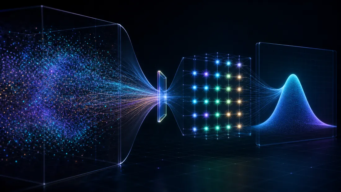
Una red neuronal Bayesian pone un prior sobre los pesos y busca el posterior . El normalizador requiere integrar sobre cada configuración de pesos, lo cual es intratable para cualquier cosa con más de un puñado de parámetros.
La inferencia variacional reemplaza el posterior intratable con una familia tratable — típicamente un Gaussiano factorizado — y minimiza
Dado que eso implica el posterior desconocido, en su lugar maximizamos el Límite Inferior de Evidencia:
El primer término empuja a explicar los datos; el segundo lo mantiene cerca del prior. Bayes by Backprop (Blundell et al., 2015) hace esto diferenciable con el truco de reparametrización: muestra , establece .
En la práctica, VI duplica el conteo de parámetros, aumenta la varianza del gradiente (cada pasada hacia adelante usa pesos diferentes), y la asunción de campo medio ignora correlaciones de pesos, lo que tiende a subestimar la incertidumbre epistémica. Para un stack de trading donde ya tienes un modelo determinista entrenado, los dos métodos más baratos abajo suelen ser el mejor punto de entrada.
Método 2: MC Dropout

Gal y Ghahramani (2016) mostraron que una red entrenada con dropout y evaluada con dropout aún activo en tiempo de prueba es un procedimiento de inferencia variacional aproximado en un proceso Gaussiano profundo. Dropout ya induce una distribución sobre subredes; mantenerlo activo durante la inferencia y ejecutar pasadas hacia adelante muestrea de ese posterior implícito.
Esto no existe en ningún otro lugar de este blog. El código publicado aquí usa dropout solo como regularizador durante el entrenamiento (modelado de spread, TFT con dropout=0.1–0.3). Mantenerlo activo durante la inferencia es un cambio de una línea con un significado completamente diferente.
Estadísticas Predictivas
Dadas pasadas hacia adelante estocásticas produciendo y varianzas por pasada :
Media predictiva:
Epistémica (desacuerdo entre pasadas):
Aleatoria (media del ruido predicho):
La descomposición es exactamente la ley de varianza total: varianza de la media condicional, más media de la varianza condicional. La varianza predictiva total es su suma.
Implementación en PyTorch
import torch
import torch.nn as nn
import numpy as np

class MCDropoutNet(nn.Module):
    """
    Red de predicción de retornos con MC Dropout para estimación de incertidumbre.
    Devuelve tanto la media predicha como log-varianza (aleatoria).
    """
    def __init__(self, input_dim: int, hidden_dim: int = 128, dropout_p: float = 0.1):
        super().__init__()
        self.net = nn.Sequential(
            nn.Linear(input_dim, hidden_dim),
            nn.ReLU(),
            nn.Dropout(p=dropout_p),
            nn.Linear(hidden_dim, hidden_dim),
            nn.ReLU(),
            nn.Dropout(p=dropout_p),
        )
        self.head_mu = nn.Linear(hidden_dim, 1)        # retorno predicho
        self.head_logvar = nn.Linear(hidden_dim, 1)    # log(varianza aleatoria)

    def forward(self, x: torch.Tensor):
        h = self.net(x)
        return self.head_mu(h), self.head_logvar(h)


def heteroscedastic_loss(mu, log_var, target):
    """Log-verosimilitud negativa para un Gaussiano con varianza aprendida, dependiente de la entrada."""
    precision = torch.exp(-log_var)
    return torch.mean(0.5 * precision * (target - mu) ** 2 + 0.5 * log_var)


@torch.no_grad()
def mc_predict(model: MCDropoutNet, x: torch.Tensor, n_samples: int = 100):
    """
    Inferencia MC Dropout: mantener dropout activo, recoger T pasadas hacia adelante,
    descomponer varianza predictiva en partes epistémica y aleatoria.
    """
    model.train()  # NO eval() — esto es lo que mantiene dropout activo
    mus, log_vars = [], []
    for _ in range(n_samples):
        mu, log_var = model(x)
        mus.append(mu)
        log_vars.append(log_var)

    mus = torch.stack(mus)            # (T, batch, 1)
    log_vars = torch.stack(log_vars)  # (T, batch, 1)

    pred_mean = mus.mean(dim=0)
    epistemic_var = mus.var(dim=0)              # Var sobre pasadas
    aleatoric_var = log_vars.exp().mean(dim=0)  # E sobre pasadas

    return {
        "mean": pred_mean.squeeze(-1),
        "epistemic_std": epistemic_var.sqrt().squeeze(-1),
        "aleatoric_std": aleatoric_var.sqrt().squeeze(-1),
        "total_std": (epistemic_var + aleatoric_var).sqrt().squeeze(-1),
    }
El entrenamiento usa la pérdida heteroscedástica, lo que hace que la cabeza de varianza signifique algo. Note la estructura autorreguladora: el término 0.5 * precision * (target - mu)**2 quiere varianza pequeña, el término 0.5 * log_var la castiga, y el punto de balance es el nivel de ruido condicional.
model = MCDropoutNet(input_dim=50, hidden_dim=128, dropout_p=0.1)
optimizer = torch.optim.AdamW(model.parameters(), lr=1e-3, weight_decay=1e-4)

for epoch in range(200):
    model.train()
    for x_batch, y_batch in train_loader:
        mu, log_var = model(x_batch)
        loss = heteroscedastic_loss(mu, log_var, y_batch)
        optimizer.zero_grad()
        loss.backward()
        optimizer.step()
El error que silenciosamente mata el método: llamar model.eval() dentro de mc_predict. Desactiva dropout, cada pasada devuelve el valor idéntico, epistemic_var colapsa a exactamente cero, y tu regla de dimensionamiento silenciosamente revierte a Kelly plano sobre varianza aleatoria. Falla sin errorar. Asegúrate de que epistemic_var > 0 en tu ruta de inferencia.
Elegir el número de pasadas hacia adelante
- : límite inferior razonable para una media estable
- : valor predeterminado utilizable para media y varianza
- : rendimientos decrecientes a menos que necesites cuantiles de cola
Método 3: Deep Ensembles

Lakshminarayanan et al. (2017) entrenan redes independientes desde diferentes inicializaciones aleatorias y agregan. A pesar de no ser formalmente Bayesian, los deep ensembles consistentemente superan métodos más principistas en benchmarks de calibración de incertidumbre.
El desacuerdo entre miembros es la estimación epistémica. Los ensembles aparecen en otro lugar de este blog como dispositivos de agregación — detección de anomalías, detección de régimen HMM, block bootstrap EnbPI conforme — pero nunca como estimador de incertidumbre vía dispersión inter-miembros. Ese es el uso aquí.
Implementación de Ensemble
La diversidad proviene del entrenamiento independiente, no de construir objetos. Un ensemble de miembros no entrenados o entrenados idénticamente devuelve ruido o varianza epistémica cero:
class DeepEnsemble:
    def __init__(self, input_dim: int, n_models: int = 5, hidden_dim: int = 128):
        self.models = []
        for seed in range(n_models):
            torch.manual_seed(seed)          # diferente init por miembro
            self.models.append(
                MCDropoutNet(input_dim, hidden_dim, dropout_p=0.0)
            )

    def fit(self, train_loader, epochs: int = 200, lr: float = 1e-3):
        """Cada miembro se entrena independientemente. Aquí es de donde viene la diversidad
        -- diferente init, diferente orden de shuffle. Saltarse esto
        resulta en epistemic_var == 0 (miembros idénticos) o ruido puro (no entrenado)."""
        for seed, model in enumerate(self.models):
            torch.manual_seed(1000 + seed)   # diferente stream de shuffle/dropout
            opt = torch.optim.AdamW(model.parameters(), lr=lr, weight_decay=1e-4)
            model.train()
            for _ in range(epochs):
                for x_batch, y_batch in train_loader:
                    mu, log_var = model(x_batch)
                    loss = heteroscedastic_loss(mu, log_var, y_batch)
                    opt.zero_grad()
                    loss.backward()
                    opt.step()
        return self

    @torch.no_grad()
    def predict(self, x: torch.Tensor):
        mus, variances = [], []
        for model in self.models:
            model.eval()                     # correcto aquí: sin muestreo dropout
            mu, log_var = model(x)
            mus.append(mu.squeeze(-1))
            variances.append(log_var.exp().squeeze(-1))

        all_mus = torch.stack(mus)
        all_vars = torch.stack(variances)

        epistemic_var = all_mus.var(dim=0)   # dispersión A TRAVÉS de miembros
        aleatoric_var = all_vars.mean(dim=0)

        return {
            "mean": all_mus.mean(dim=0),
            "epistemic_std": epistemic_var.sqrt(),
            "aleatoric_std": aleatoric_var.sqrt(),
            "total_std": (epistemic_var + aleatoric_var).sqrt(),
        }
Note que model.eval() es correcto en DeepEnsemble.predict y equivocado en mc_predict. La fuente de estocasticidad difiere: los ensembles la obtienen del entrenamiento independiente, MC Dropout de máscaras dropout en vivo.
Trade-offs: MC Dropout vs Deep Ensembles
| MC Dropout | Deep Ensembles | |
|---|---|---|
| Costo de entrenamiento | 1x (modelo único) | x ( modelos) |
| Costo de inferencia | pasadas hacia adelante | pasadas hacia adelante |
| Memoria | 1x parámetros | x parámetros |
| Calidad de incertidumbre | Tiende a subestimar epistémico | Mejor calibrado en general |
| Facilidad de implementación | Trivial (cambiar una bandera) | Trivial (entrena modelos) |
| Paralelismo | Pasadas secuenciales (mismo modelo) | Embarassingly paralelo |
Un híbrido pragmático: entrena un ensemble pequeño () donde cada miembro también usa MC Dropout, capturando tanto desacuerdo inter-modelo como estocasticidad intra-modelo.
El beneficio: Dimensionamiento asimétrico
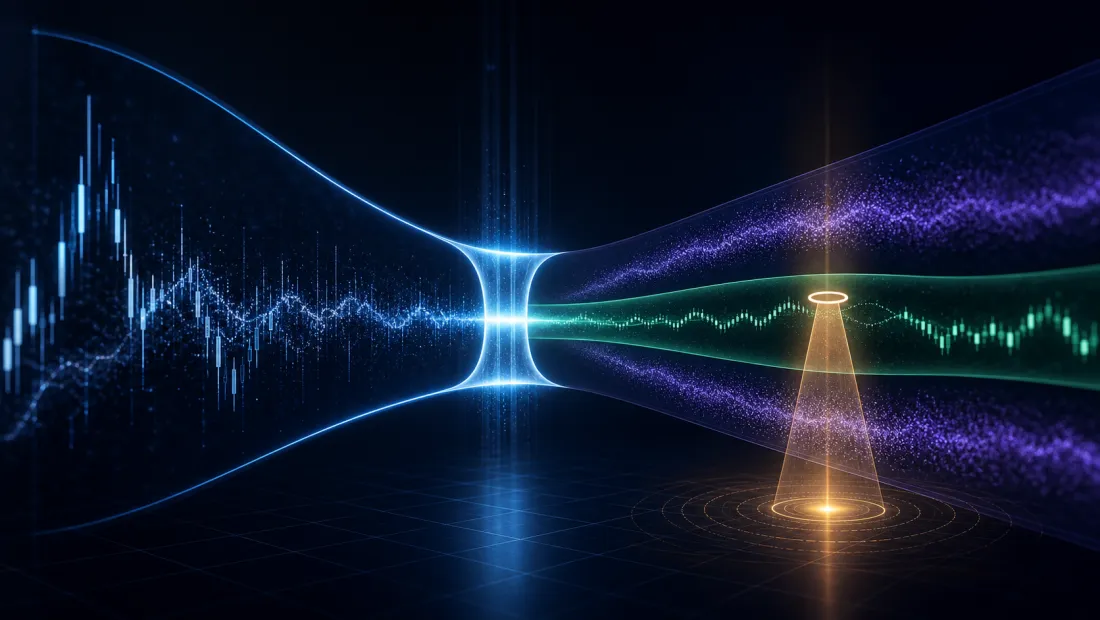
Aquí está la contribución real. Kelly Gaussiano es ; la derivación, la parábola de crecimiento, la tabla de probabilidades de drawdown y las cuatro razones para ejecutar Kelly fraccionario en lugar de completo están todas en El Criterio de Kelly para Estrategias, y no se repiten aquí. Toma a una fracción de cuarto-Kelly como dado.
La modificación es el denominador. En lugar de varianza predictiva total:
El argumento para : la varianza aleatoria es el ruido del mercado, está preciada, y soportarla es cómo gana una estrategia. La varianza epistémica es tu ignorancia — no lleva prima, y peor, está correlacionada con tu estimación estando equivocada. Cuando es grande, el numerador de Kelly es poco confiable al mismo tiempo que el denominador, así que el error de dimensionamiento se compone. Penalizarla sobrelinealmente respecto al ruido de mercado es la expresión directa de eso.
def uncertainty_adjusted_position_size(
    pred_mean: float,
    epistemic_std: float,
    aleatoric_std: float,
    max_position: float = 1.0,
    lam: float = 2.0,                   # penalización epistémica; sintoniza en validación
    max_epi_ratio: float = 0.5,         # abstente por encima de este ratio epi/alea
    base_kelly_fraction: float = 0.25,
) -> float:
    """Dimensionamiento Kelly donde la varianza epistémica se penaliza más fuerte que la aleatoria."""
    effective_var = aleatoric_std ** 2 + lam * epistemic_std ** 2
    if effective_var < 1e-10:
        return 0.0

    position = (pred_mean / effective_var) * base_kelly_fraction

    epi_ratio = epistemic_std / (aleatoric_std + 1e-8)
    if epi_ratio > max_epi_ratio:
        position *= max(0.0, 1.0 - epi_ratio)

    return float(np.clip(position, -max_position, max_position))
La compuerta merece una nota. Cero posiciones por debajo de un umbral de confianza no es nuevo aquí — el artículo conforme especifica y codifica el filtro general no-trade como con un umbral min_edge, incluyendo cómo elegir el umbral y la lectura geométrica de un intervalo que cruza cero. Ver predicción conforme para esa maquinaria. Lo que sí es nuevo es el denominador: hacer gate en dispara específicamente cuando el modelo está más confundido sobre sus propios parámetros de lo que el mercado está ruidoso — un estado que el gate de incertidumbre total no puede detectar, porque un régimen tranquilo pero desconocido puede tener baja varianza total y un ratio epistémico terrible.
Calibración: Delega esto
Una estimación de incertidumbre solo es útil si está calibrada: un intervalo nominal del 95% debería contener la verdad ~95% del tiempo. No implementes tu propia verificación de confiabilidad de cuantil Gaussiano — un intervalo paramétrico en residuos de retorno de cola pesada es exactamente el modo de fallo que predicción conforme existe para evitar, y envía un evaluate() funcional que reporta objetivo vs cobertura empírica con una garantía de muestra finita detrás. El post de TFT hace el mismo punto para cabezas de cuantil.
Re-escalado post-hoc ( ajustado en un conjunto de validación) es la solución barata, y es el primo menor de la Inferencia Conforme Adaptativa, que mantiene un nivel de fallo de cobertura en línea con un límite de cobertura de largo plazo en lugar de un re-escalado estático. ACI es la opción más fuerte; la única razón para preferir re-escalado lineal es que preserva el ratio epistémico/aleatorio, que el ancho único de ACI no hace.
Qué debe medirse antes de publicar esto
Los métodos de arriba están establecidos. La afirmación de que la división compra algo en trading no lo está, y este blog no publica reglas de dimensionamiento solo en argumentos. La barrera:
1. Conjunto de datos y objetivo. Nombra el instrumento, tamaño de vela, rango de fechas explícito, conjunto de características y objetivo de predicción.
2. La división misma. Qué fracción de varianza predictiva total es epistémica vs aleatoria, y cómo se mueve ese ratio entre una ventana tranquila nombrada y una volátil nombrada. Esta es la tabla de dinero y aún no existe. La hipótesis que vale la pena falsificar: el ratio se dispara antes que la volatilidad realizada, porque la unfamiliaridad precede a la turbulencia.
3. Cobertura vs conforme. Cobertura medida fuera de muestra de intervalos MC Dropout contra nominal, comparada con intervalos split-conforme del artículo publicado en los mismos datos. Ese enfrentamiento directo es en sí mismo un resultado nuevo y el puente natural entre los dos posts.
4. ¿Compra algo? Barrer la penalización epistémica en validación y reportar PnL y drawdown máximo contra la línea base . Si no compra nada, di así — El Negativo Honesto es la plantilla para ese resultado y es un resultado publicable.
5. Costo de inferencia. Medido, en el hardware objetivo, en cada .
Cualquier evaluación aquí se ejecuta bajo disciplina de optimización walk-forward — es un hiperparámetro, y un sintonizado en la muestra completa no es un resultado.
Consejos prácticos para producción
1. Calienta el prior. Con inferencia variacional, inicializa la media variacional desde una red determinista pre-entrenada en lugar de al azar. Típicamente reduce a la mitad el tiempo de convergencia.
2. Vigila el colapso de varianza. Las varianzas aprendidas pueden derivar hacia casi cero, revirtiendo silenciosamente el BNN a una red determinista. Monitorea la media durante el entrenamiento; añade recocido KL si es necesario.
3. Recalibra sobre una base rodante, no en un conjunto de validación fijo. Los mercados son no estacionarios y una calibración ajustada una vez decae. O reentrena sobre una ventana rodante bajo disciplina walk-forward, o deja que ACI absorba la obsolescencia del modelo en línea — el post conforme cubre el trade-off de frecuencia de reentrenamiento directamente.
4. La diversidad del ensemble importa. Diferentes semillas, diferentes shuffles, opcionalmente diferentes hiperparámetros por miembro. La diversidad de inicialización es el conductor primario de calidad del ensemble, por lo que el bucle fit() arriba no es opcional.
5. Registra la descomposición, no solo el total. Almacena ambos componentes junto con resultados realizados. Sin esto no puedes responder la única pregunta que importa en revisión: cuando el dimensionador redujo exposición, ¿fue porque el mercado estaba ruidoso o porque el modelo estaba perdido — y tuvo razón?
6. Incertidumbre como característica. Las estadísticas epistémicas rodantes pueden ser ellas mismas predictivas de drawdowns. Plausible, no medido, y vale un post separado.
Limitaciones y advertencias honestas
- Los posteriors aproximados siguen siendo aproximados. MC Dropout y VI dan una vista limitada del posterior verdadero. Mejor que nada, no verdad fundamental, y no hay garantía de cobertura unida a ninguno.
- La calibración se degrada exactamente cuando la necesitas. En un régimen verdaderamente nuevo el modelo todavía puede estar miscalibrado — solo tiende a estar menos miscalibrado que uno determinista. Las estimaciones de incertidumbre de una entrada fuera de distribución son ellas mismas salidas fuera de distribución.
- La varianza aleatoria puede absorber señal epistémica. Si la cabeza heteroscedástica es lo suficientemente flexible, aprende a explicar la incertidumbre del modelo como ruido de datos, colapsando hacia cero y derrotando silenciosamente toda la descomposición. Este es el modo de fallo más importante en este post y no se anuncia a sí mismo. Monitorea el ratio a través de regímenes; un ratio que nunca se mueve es una descomposición rota, no un mercado estable.
- es un parámetro libre. Introducir una perilla ajustable en una regla de dimensionamiento es cómo se construyen reglas de dimensionamiento sobreajustadas. Necesita una justificación walk-forward o necesita fijarse en 1.
Conclusión
La predicción conforme ya da a este blog anchos de intervalo con garantía de cobertura, y Kelly ya le da una regla de dimensionamiento. Lo que ninguno da es una respuesta a por qué el intervalo es ancho. Dividir la varianza predictiva en partes epistémicas y aleatorias responde eso, y la respuesta es accionable de una forma que el total no lo es: el ruido de mercado es riesgo compensado, la ignorancia del modelo no lo es, y el denominador de dimensionamiento debería decirlo.
MC Dropout hace la división casi gratuita — una línea (model.train() en inferencia) convierte cualquier red dropout en una Bayesian aproximada. Los deep ensembles cuestan x y calibran mejor. Ambos alimentan el mismo denominador asimétrico .
Si realmente paga es una pregunta empírica que este borrador aún no responde. Las medidas listadas arriba son el precio de publicarlo.
Referencias:
- Blundell, C., Cornebise, J., Kavukcuoglu, K., & Wierstra, D. (2015). Weight Uncertainty in Neural Networks. ICML.
- Gal, Y. & Ghahramani, Z. (2016). Dropout as a Bayesian Approximation: Representing Model Uncertainty in Deep Learning. ICML.
- Lakshminarayanan, B., Pritzel, A., & Blundell, C. (2017). Simple and Scalable Predictive Uncertainty Estimation using Deep Ensembles. NeurIPS.
- Kendall, A. & Gal, Y. (2017). What Uncertainties Do We Need in Bayesian Deep Learning for Computer Vision? NeurIPS.
- Gibbs, I. & Candes, E. (2021). Adaptive Conformal Inference Under Distribution Shift. NeurIPS.
- Kelly, J. L. (1956). A New Interpretation of Information Rate. Bell System Technical Journal.
Authors
Trading-systems engineer
Trading-systems engineer building bots since 2017: cross-exchange arbitrage (connected up to 30 venues), cointegration-based pairs arbitrage across spot and futures, scalping, news and sentiment-driven strategies, trend algorithms, and portfolio management and balancing algorithms. Also builds sub-millisecond order execution, big-data warehouses, backtesting engines, AI agents, and trading interfaces (incl. open-source profitmaker.cc). Stack: JS/TS, Python, Rust/Zig/Go, DevOps, backend, frontend, architecture.
Read More
Predicción conforme para el dimensionamiento de posiciones consciente del riesgo

Procesos gaussianos para modelado de precios no paramétrico