Tổn thất tạm thời và LVR: toán học thực sự về lợi nhuận của LP

Cung cấp thanh khoản trông giống như một sản phẩm lợi suất và hoạt động giống như một cuốn sách quyền chọn ngắn hạn. Tiêu đề APR trên bảng điều khiển nhóm là một con số tổng: nó tính phí chảy vào và âm thầm bỏ qua hai chi phí chảy ra — sự khác biệt giữa vị thế của bạn trở thành gì và những gì bạn đã gửi (tổn thất vô thường), và sự chảy máu ổn định, lén lút hơn đối với các nhà kinh doanh chênh lệch giá, những người chọn ra các báo giá cũ của bạn trên mỗi biến động giá (tổn thất so với tái cân bằng). Nếu tính toán đúng, toàn bộ hoạt động kinh doanh sẽ giảm xuống một bất đẳng thức: liệu dòng phí có bù đắp được chi phí biến động của việc nắm giữ vị thế không? Nếu tính toán sai, bạn là người bán phương sai một cách có hệ thống mà quên định giá phương sai.
Bài viết này là phần tiếp theo đã hứa của Uniswap v3 dành cho các nhà định lượng, kết thúc bằng việc đặt tên tổn thất so với tái cân bằng và chỉ ra ở đây. Chúng tôi xây dựng phép tính lợi nhuận từ các nguyên tắc cơ bản: dạng đóng của tổn thất vô thường trên một nhóm sản phẩm không đổi, tại sao thanh khoản tập trung là IL được đòn bẩy, kết quả LVR σ²/8 và sự phân tách PnL chính xác mà nó cho phép, cách đo lường lựa chọn bất lợi theo kinh nghiệm theo từng khối, và điều kiện hòa vốn — so sánh phí với biến động — cho bạn biết khi nào một vị thế LP thực sự là +EV so với việc chỉ nắm giữ các token.
Bất biến sản phẩm không đổi và sự ra đời của tổn thất vô thường
Một nhóm Uniswap v2 giữ các khoản dự trữ của token rủi ro và của numéraire và thực thi trên mỗi giao dịch. Giá biên của tài sản rủi ro là . Bởi vì được bảo toàn, các khoản dự trữ ở bất kỳ mức giá nào đều được cố định:
Bắt đầu ở mức giá với các khoản dự trữ và để giá trôi đến . Vị thế của LP có giá trị, được đánh dấu ở mức giá mới,
Nếu bạn chỉ đơn giản giữ các token đã gửi thay vì gộp chúng, bạn sẽ có giá trị
Xác định tỷ lệ giá . Chia, và và triệt tiêu sạch sẽ, để lại tổn thất vô thường như một hàm của tỷ lệ giá một mình:
Đó là toàn bộ đối tượng. Nó âm đối với mọi và bằng không chỉ khi giá trở lại nơi bạn đã nhập — "vô thường" chính xác vì nó biến mất nếu giá quay trở lại. Hai thuộc tính đáng được nội hóa.
Nó đối xứng theo log-giá. Thay thế : biểu thức không thay đổi, vì . Một lần tăng gấp đôi và một lần giảm một nửa đều gây tổn thất như nhau. Cụ thể, một biến động 2× () và một biến động −50% () đều cho
Sự đối xứng rõ ràng nhất khi bạn viết tỷ lệ giá theo logarit. Với , một thao tác ngắn gọn sẽ làm cho IL sụp đổ thành một secant hyperbolic:
điều này làm cho hình dạng bậc hai theo log-lợi nhuận trở nên rõ ràng: gần giá nhập, IL tăng theo bình phương của biến động giá logarit — dấu hiệu của một khoản thanh toán gamma ngắn hạn, và lý do nó vẫn không đáng kể đối với các biến động nhỏ và gây tổn thất lớn đối với các xu hướng.
| Tỷ lệ giá | Biến động | IL so với HODL |
|---|---|---|
| 0.50 | −50% | −5.72% |
| 0.70 | −30% | −1.57% |
| 0.90 | −10% | −0.14% |
| 1.00 | ổn định | 0.00% |
| 1.10 | +10% | −0.11% |
| 1.50 | +50% | −2.02% |
| 2.00 | 2× | −5.72% |
| 4.00 | 4× | −20.0% |

Các con số có vẻ nhỏ cho đến khi bạn nhớ chúng đo lường điều gì: IL là khoảng cách so với việc nắm giữ, và nó chỉ được hiện thực hóa tương đối so với tiêu chuẩn đó. Một token tăng gấp 4 lần vẫn khiến LP tăng rất nhiều về mặt đô la — chỉ ít hơn 20% so với nếu họ đã nắm giữ. IL không phải là một khoản lỗ bạn cảm thấy; đó là một chi phí cơ hội bạn phải được trả để chịu đựng. Dòng phí là khoản thanh toán đó. Liệu nó có đủ hay không là phần còn lại của bài viết này.
Thanh khoản tập trung là tổn thất vô thường được đòn bẩy
Uniswap v3 cho phép LP giới hạn vốn trong một phạm vi giá . Trong phạm vi đó, vị thế hoạt động chính xác như một nhóm v2 — cùng một đường cong liên kết — nhưng chỉ sử dụng các khoản dự trữ cần thiết để bao phủ dải đó (cấu trúc dự trữ ảo được suy ra trong bài viết về cơ chế v3). Hậu quả đối với IL rất rõ ràng, và nó xuất phát từ một dòng đại số.
Viết . Một vị thế v3 với thanh khoản trên , được nhập ở mức giá và vẫn trong phạm vi ở , giữ và . Tính giá trị của nó trừ đi giá trị HODL của các token ban đầu của nó, và mọi thứ liên quan đến và đều triệt tiêu:
Đây là cùng một tổn thất phân kỳ tuyệt đối như một nhóm v2 với giống hệt — các giới hạn phạm vi không xuất hiện. Vậy thì sự đau đớn tăng thêm đến từ đâu? Từ vốn. Tập trung vào cho phép cùng một số đô la hỗ trợ một lớn hơn nhiều. Đối với một phạm vi được căn giữa hình học trên giá nhập, hệ số khuếch đại chính xác là
hệ số nhân "hiệu quả vốn" của v3. Một vị thế toàn dải có ; một dải từ đến cho ; một dải quanh (±10%) cho . Bởi vì tổn thất tuyệt đối tỷ lệ với và vốn bằng nhau mua lần nhiều hơn, IL phân số tỷ lệ theo cùng một cách:
Lấy vị thế ±10% đó, giá nhập $3.000, và tăng giá lên. Các con số v2 từ bảng trên được nhân với ~20:
| Giá | Biến động | v2 IL | v3 IL () |
|---|---|---|---|
| 3.150 | +5% (trong phạm vi) | −0.030% | −0.61% |
| 3.300 | +10% (ở giới hạn trên) | −0.11% | −2.32% |
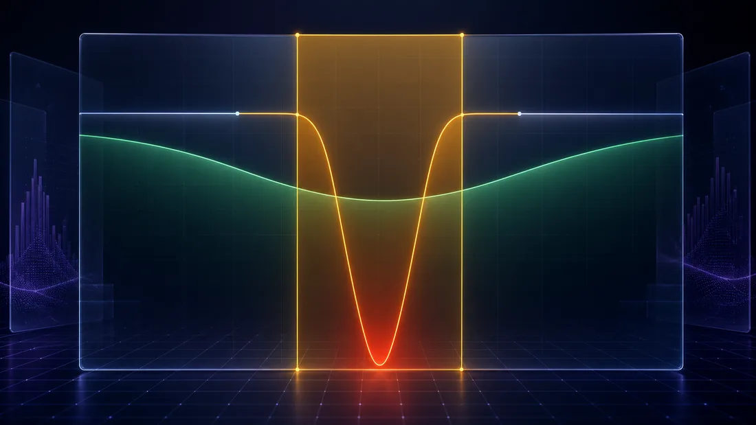
Một biến động 10% khiến LP toàn dải mất 11 điểm cơ bản, khiến LP tập trung mất 2,3% so với việc nắm giữ. Và nó còn tệ hơn ở ranh giới, bởi vì phạm vi có một cạnh thứ hai mà công thức trên che giấu: một khi giá vượt qua , vị thế là 100% numéraire, ngừng kiếm phí và sự phân kỳ của nó đóng băng ở thành phần ranh giới. LP tập trung đã bán hoàn toàn tài sản rủi ro khi giá tăng và giờ đây theo dõi bất kỳ đợt tăng giá nào tiếp theo mà không có nó — đuôi straddle ngắn, bị khóa, với dòng phí bị tắt. Tập trung là đòn bẩy đối với cả thu nhập phí và tổn thất, cộng với sự phụ thuộc vào đường đi — thời gian trong phạm vi — mà tỷ lệ ngây thơ không nắm bắt được.
LVR: tổn thất bạn không thể đổ lỗi cho thị trường
Tổn thất vô thường đo lường LP so với một HODLer thụ động, và tiêu chuẩn đó âm thầm đưa vào rủi ro thị trường: hầu hết những gì "IL so với HODL" tính phí bạn chỉ là rủi ro định hướng mà bạn sẽ phải chịu đựng dù sao bằng cách sở hữu các token. Sự phân tách sắc nét hơn — cái cô lập chi phí đặc trưng của việc là một AMM — là tổn thất so với tái cân bằng (LVR), từ Milionis, Moallemi, Roughgarden và Zhang, Tạo lập thị trường tự động và tổn thất so với tái cân bằng (arXiv:2208.06046).
Ý tưởng là để đánh giá LP không phải so với việc nắm giữ, mà so với một danh mục đầu tư tái cân bằng nắm giữ, tại mỗi thời điểm, chính xác cùng một lượng token như nhóm — cùng delta, cùng rủi ro thị trường — nhưng giao dịch ở mức giá thị trường bên ngoài không ma sát thay vì chống lại đường cong liên kết của nhóm. Cả hai danh mục đầu tư đều mang rủi ro giá giống hệt nhau, vì vậy việc trừ cái này khỏi cái kia sẽ loại bỏ hoàn toàn nhiễu thị trường và chỉ để lại chi phí cấu trúc của việc là AMM: số tiền mà nhóm mất vì các nhà kinh doanh chênh lệch giá, chứ không phải LP, nắm bắt mọi biến động giá. Phần còn lại đó là LVR.
Mô hình hóa giá bên ngoài dưới dạng chuyển động Brown hình học với biến động . Kết quả trung tâm của bài báo — mà các tác giả gọi là "công thức Black–Scholes cho AMM" — là LVR tích lũy dưới dạng một sự trôi dạt xác định, không âm:
trong đó là lượng tài sản rủi ro của nhóm dưới dạng hàm của giá và (AMM bán tài sản rủi ro khi giá tăng). Đối với nhóm sản phẩm không đổi, , vì vậy , và vì giá trị nhóm là , tỷ lệ dưới dạng phần trăm giá trị nhóm sụp đổ thành một hằng số:
Đó là σ²/8 nổi tiếng. Nó không phụ thuộc vào phí và không phụ thuộc vào hàng tồn kho: một nhóm sản phẩm không đổi mất giá trị của nó mỗi đơn vị thời gian do kinh doanh chênh lệch giá, chấm hết. Với biến động hàng ngày 5%, đó là điểm cơ bản mỗi ngày — khoảng 11% giá trị nhóm mỗi năm — trước khi một đô la phí nào được tính. Đối với một vị thế tập trung, logic tương tự cho trong phạm vi: đòn bẩy khuếch đại IL cũng khuếch đại LVR bằng cùng một yếu tố.
Tại sao LVR là đơn vị tài khoản đúng, và IL thì không, là do một thuộc tính: sự khác biệt giữa LP và tái cân bằng có biến động bằng không. Đó là một sự trôi dạt có thể dự đoán được thuần túy, . Điều đó có nghĩa là rủi ro giá có thể được phòng ngừa hoàn toàn — tái tạo danh mục đầu tư tái cân bằng bằng một phòng ngừa delta động và những gì còn lại là xác định. Do đó, kinh tế học thực sự của LP là
Phòng ngừa thuật ngữ đầu tiên và LP còn lại phí − LVR − gas — một vị thế phương sai ngắn hạn có lợi nhuận là dòng phí và chi phí của nó là một sự chảy máu liên tục, có thể dự đoán được, do biến động. Đây chính xác là sự đánh đổi gamma-theta của một cuốn sách quyền chọn ngắn hạn: LVR là chi phí gamma , phí là theta bạn thu thập, và sự tương tự với định giá quyền chọn Black–Scholes là cấu trúc, không phải trang trí. Nó cũng là cùng một căng thẳng lựa chọn bất lợi so với chênh lệch mà Avellaneda–Stoikov chính thức hóa cho các nhà tạo lập thị trường sổ lệnh, với cấp phí của nhóm đóng vai trò là chênh lệch được báo giá.
Một sự tinh chỉnh giữ cho khung trung thực. σ²/8 sạch sẽ giả định kinh doanh chênh lệch giá liên tục, không tốn kém. Trong thực tế, cấp phí tự nó tạo ra một dải không kinh doanh chênh lệch giá — các nhà kinh doanh chênh lệch giá chỉ giao dịch khi biến động giá vượt quá phí — vì vậy LVR thực tế nhỏ hơn con số không ma sát, và phí có hai nhiệm vụ: chúng trả tiền cho bạn và chúng mở rộng dải bảo vệ bạn. Phiên bản có phí, thời gian rời rạc được giải quyết trong phần tiếp theo Tạo lập thị trường tự động và lợi nhuận kinh doanh chênh lệch giá khi có phí (Milionis, Moallemi, Roughgarden, 2023); coi σ²/8 liên tục là giới hạn trên của sự chảy máu.

Markout: đo lường lựa chọn bất lợi từng khối
LVR là một định lý về sự khuếch tán. Bóng tối thực nghiệm mà nó tạo ra trên các giao dịch thực tế là markout, và đó là cách bạn đo lường lựa chọn bất lợi trên một vị thế trực tiếp mà không cần bất kỳ mô hình biến động nào.
Markout đánh giá một giao dịch so với một giá "công bằng" tham chiếu một khoảng thời gian sau đó. Đối với một nhà cung cấp thanh khoản thụ động, mọi giao dịch hoán đổi chống lại phạm vi của bạn là một giao dịch bạn không chọn — người nhận đã chọn nó, và họ chọn nó vì nó tốt cho họ. Xác định markout của LP trên một giao dịch là sự thay đổi hàng tồn kho đã ký nhân với biến động giá sau đó:
trong đó là số lượng tài sản rủi ro mà LP đã mua trong giao dịch (âm khi LP bán). Dòng chảy có thông tin và độc hại làm cho điều này có hệ thống âm: nhóm mua tài sản rủi ro từ một người bán đúng, ngay trước khi giá giảm, và bán cho một người mua đúng, ngay trước khi nó tăng. Trung bình trên nhiều giao dịch, LP ở phía sai của tick tiếp theo — đó chính xác là LVR được hiện thực hóa từng giao dịch một.
Được đo theo từng khối, điều này trở thành một chỉ số lựa chọn bất lợi rõ ràng: lấy sự thay đổi hàng tồn kho ròng của LP trong một khối và đánh dấu nó so với giá một hoặc vài khối sau đó. Tổng hợp trong suốt vòng đời của một vị thế, tổng các markout theo từng khối là LVR thực nghiệm. Lý do nó quan trọng là vì con số markout thường xấu xí. Các nghiên cứu thực nghiệm mẫu lớn — bắt đầu với phân tích năm 2021 của Loesch, Hindman, Richardson và Welch về các vị thế Uniswap v3 (nghiên cứu Topaze Blue / Bancor) và được củng cố bởi các bảng điều khiển định lượng LVR sau đó — đã phát hiện ra rằng một phần lớn các LP v3, trên nhiều nhóm lớn khoảng một nửa hoặc hơn, hoạt động kém hơn so với việc chỉ nắm giữ các token một khi IL và lựa chọn bất lợi được tính vào phí. Cartea, Drissi và Monga chính thức hóa cùng một lượng cho thanh khoản tập trung là "tổn thất có thể dự đoán được," đạt được cùng một sự trôi dạt tỷ lệ với biến động bằng một con đường khác.
Bài học thực tế cho một LP giám sát một sổ lệnh trực tiếp: APR phí là một con số tổng; phí + markout là con số ròng. Một vị thế có thể cho thấy lợi suất phí lành mạnh và markout âm sâu, và tổng là những gì bạn thực sự kiếm được. Các nhà kinh doanh chênh lệch giá hiện thực hóa markout đó chống lại bạn là những người tìm kiếm tương tự được mô tả trong bài viết về MEV và mempool — một cuộc tấn công ngược lại một báo giá AMM cũ sau mỗi biến động oracle là việc trích xuất LVR, từng khối một, và đó là phần cuối lành tính, điều chỉnh giá của phổ MEV ngay cả khi đó là phần cuối độc hại của PnL của bạn.

Khi LPing thực sự đánh bại việc nắm giữ
Thu gọn mọi thứ vào quyết định mà nó phục vụ. Phòng ngừa rủi ro thị trường và một vị thế LP là +EV so với tiêu chuẩn của nó chính xác khi tỷ lệ thu nhập phí bù đắp tỷ lệ LVR:
trong đó là cấp phí của nhóm và là doanh thu — khối lượng giao dịch chia cho TVL, mỗi đơn vị thời gian. Sắp xếp lại, điều kiện là một so sánh hai biến động. Dòng phí ngụ ý một biến động hòa vốn
và LP thắng bất cứ khi nào biến động thực tế thấp hơn nó. Đây là phiên bản của AMM về biến động ngụ ý so với thực tế: nhóm báo giá một biến động ngụ ý thông qua lợi suất phí của nó, và việc cung cấp thanh khoản là bán phương sai ở mức đó. Một số điểm tham chiếu đã được tính toán (doanh thu rõ ràng là giả định, được chọn để đại diện cho các nhóm hoạt động):
- Nhóm 0,05%, doanh thu 1,0/ngày (khối lượng ≈ TVL hàng ngày): hàng ngày. Dưới ~6,3% biến động hàng ngày thực tế, LP có lợi.
- Nhóm 0,30%, doanh thu 0,2/ngày: hàng ngày.
- Stablecoin / cặp tương quan, hàng ngày: LVR là mỗi ngày — về cơ bản là không có gì, bởi vì LVR tỷ lệ với bình phương của biến động. Hầu hết mọi lợi suất phí đều bù đắp được nó.
Sự phụ thuộc bình phương đó là toàn bộ chiến lược trong một sự thật. Giảm một nửa biến động của cặp sẽ giảm một phần tư sự chảy máu, trong khi lợi suất phí không bị ảnh hưởng. Đó là lý do tại sao lợi thế LP bền vững nằm ở các cặp có σ thấp — các cặp stablecoin, các cặp token đặt cược thanh khoản/ETH và các chân tương quan chặt chẽ khác — và tại sao LPing cặp biến động là một đặt cược rằng phí là phi thường hoặc bạn có thể phòng ngừa và tái cân bằng nhanh hơn nhóm chảy máu.
import numpy as np

def breakeven_daily_vol(fee_tier: float, turnover: float) -> float:
    """Daily volatility at which fee income exactly offsets v2 (or in-range v3) LVR.
    fee_tier: pool fee as a fraction (0.0005 = 0.05%).
    turnover: daily trading volume / TVL."""
    daily_fee_yield = fee_tier * turnover
    return np.sqrt(8 * daily_fee_yield)

def lp_is_plus_ev(fee_tier, turnover, sigma_forecast) -> bool:
    """LP beats the rebalancing benchmark iff forecast vol < break-even vol."""
    return sigma_forecast < breakeven_daily_vol(fee_tier, turnover)

sigma_star = breakeven_daily_vol(0.0005, 1.0)   # ~0.063  (6.3%/day)
lp_is_plus_ev(0.0005, 1.0, sigma_forecast=0.045)  # 4.5% forecast -> True
Đầu vào duy nhất mà toàn bộ quyết định phụ thuộc vào là — không phải biến động thực tế của tháng trước, mà là dự báo biến động thực tế trong suốt thời gian nắm giữ, đó chính xác là một vấn đề dự báo biến động. Một dự báo biến động GARCH một ngày trước được đưa vào biến "nhóm này có trả đủ không" thành một tín hiệu trực tiếp, có thể cập nhật: LP khi dự báo nằm dưới điểm hòa vốn, đứng ngoài khi một sự thay đổi chế độ biến động đẩy nó lên trên.
Sự tập trung không làm thay đổi tỷ lệ khi bạn ở trong phạm vi — nó nhân lợi suất phí và LVR với cùng một , vì vậy bất đẳng thức phí so với biến động là bất biến theo tỷ lệ trong phạm vi. Điều nó thay đổi là mọi thứ xung quanh các cạnh: một phạm vi hẹp dành ít thời gian hơn trong phạm vi (không có phí, IL đóng băng khi ra ngoài), và đòi hỏi tái cân bằng tích cực mà gas và markout tái nhập là những chi phí thực tế. Vì vậy, quy tắc trung thực cho các phạm vi hẹp là hẹp: chỉ biện minh cho chúng khi dự báo biến động thực tế của bạn thấp so với chiều rộng phạm vi, hoặc khi bạn đang tích cực quản lý và phòng ngừa vị thế thay vì thiết lập và quên nó. Cơ chế của việc quản lý tích cực đó — các yếu tố kích hoạt tái cân bằng, phòng ngừa delta đối với hàng tồn kho thay đổi của nhóm và biến phí − LVR thành một chiến lược được phòng ngừa — là chủ đề của bài viết đi kèm về các chiến lược LP Uniswap v3 và phòng ngừa.
Những điều cần ghi nhớ
- Tổn thất vô thường có dạng đóng, , đối xứng theo log-giá (một biến động 2× và một biến động −50% đều có chi phí 5,72%) và bậc hai theo log-lợi nhuận gần điểm nhập — dấu hiệu của một khoản thanh toán gamma ngắn hạn.
- Thanh khoản tập trung là IL được đòn bẩy. Tổn thất phân kỳ tuyệt đối không thay đổi đối với một nhất định, nhưng vốn bằng nhau triển khai lần nhiều hơn, vì vậy cả IL và phí đều tỷ lệ với — và vị thế đóng băng thành tài sản thua lỗ một khi giá thoát khỏi phạm vi.
- LVR là tổn thất tồn tại sau khi phòng ngừa. Được đánh giá so với một danh mục đầu tư tái cân bằng, một nhóm sản phẩm không đổi mất giá trị mỗi đơn vị thời gian bất kể phí; PnL được phòng ngừa của LP là phí − LVR − gas, một khoản lợi nhuận phương sai ngắn hạn.
- Markout là LVR được đo trên các giao dịch thực tế. Markout theo từng khối định lượng trực tiếp lựa chọn bất lợi, và hồ sơ thực nghiệm cho thấy một phần lớn các LP v3 có lợi nhuận ròng âm so với việc nắm giữ một khi nó được tính. APR phí là tổng; phí + markout là ròng.
- Quyết định là một bất đẳng thức. Một LP đánh bại tiêu chuẩn của nó khi lợi suất phí vượt quá , tức là khi biến động thực tế giảm xuống dưới điểm hòa vốn ngụ ý phí . Bởi vì LVR tỷ lệ với , lợi thế nằm ở các cặp có biến động thấp, tương quan — và đầu vào quyết định nó là một dự báo biến động.
Tài liệu tham khảo
- Milionis, J., Moallemi, C. C., Roughgarden, T., Zhang, A. L. (2022). Tạo lập thị trường tự động và tổn thất so với tái cân bằng. arXiv:2208.06046.
- Milionis, J., Moallemi, C. C., Roughgarden, T. (2023). Tạo lập thị trường tự động và lợi nhuận kinh doanh chênh lệch giá khi có phí. arXiv:2305.14604.
- Loesch, S., Hindman, N., Richardson, M. B., Welch, N. (2021). Tổn thất vô thường trong Uniswap v3. Topaze Blue / Bancor.
- Cartea, Á., Drissi, F., Monga, M. (2023). Tài chính phi tập trung và tạo lập thị trường tự động: Tổn thất có thể dự đoán được và cung cấp thanh khoản tối ưu. SSRN / arXiv.
- Adams, H., Zinsmeister, N., Salem, M., Keefer, R., Robinson, D. (2021). Uniswap v3 Core (sách trắng).
- Fan, Z., Marmolejo-Cossío, F., Moroz, D., Neuder, M., Rao, R., Parkes, D. C. (2022). Cung cấp thanh khoản chiến lược trong Uniswap v3. arXiv:2106.12033.
Tác Giả
Trading-systems engineer
Trading-systems engineer building bots since 2017: cross-exchange arbitrage (connected up to 30 venues), cointegration-based pairs arbitrage across spot and futures, scalping, news and sentiment-driven strategies, trend algorithms, and portfolio management and balancing algorithms. Also builds sub-millisecond order execution, big-data warehouses, backtesting engines, AI agents, and trading interfaces (incl. open-source profitmaker.cc). Stack: JS/TS, Python, Rust/Zig/Go, DevOps, backend, frontend, architecture.
Đọc Thêm

Active Uniswap v3 LPing as Market Making: Range Selection, Rebalancing, and Delta Hedging

Uniswap v3 cho Quant: Thanh khoản Tập trung và Toán học Tick từ Nguyên lý Cơ bản