Physics-Informed Neural Networks for Options Pricing

Интересная часть применения PINN к деривативам связана не с Black-Scholes. Для Black-Scholes есть замкнутая формула; сеть, которая ее воспроизводит, служит проверкой здравого смысла, а не результатом. Интересно все, для чего замкнутой формулы нет и где конечные разности упираются в ограничения: двумерное уравнение Heston со смешанной производной , задача со свободной границей для американского опциона и частичное интегро-дифференциальное уравнение Мертона, интегральный член которого связывает каждую точку области со всеми остальными.
В этой статье показано, как каждый из этих случаев превращается в функцию потерь. Конкретно: невязка в логарифме цены, благодаря которой PINN для Black-Scholes становится обучаемой; сеть Heston с тремя входами, для которой смешанная производная автоматически получается через autograd; подход со штрафом и подход с двумя сетями для досрочного исполнения; а также квадратура Гаусса - Эрмита, помещающая интеграл скачков внутрь невязки PDE.
Это не бенчмарк. Каждое число ниже, похожее на результат, является либо целевым ориентиром, либо ссылкой, и помечено соответственно. План измерений приведен в конце.
PINN были представлены в работе Raissi et al. (2019), а механика уже разобрана в этом блоге в статье Задача Навье - Стокса, где тот же прием с autograd-невязкой используется для поиска сингулярностей в уравнениях жидкости: PDE становится членом функции потерь, autodiff дает точные производные сети по ее входам, и сетка вообще не строится. Здесь меняется только PDE, входящее в функцию потерь.
PDE Black-Scholes как физическое ограничение
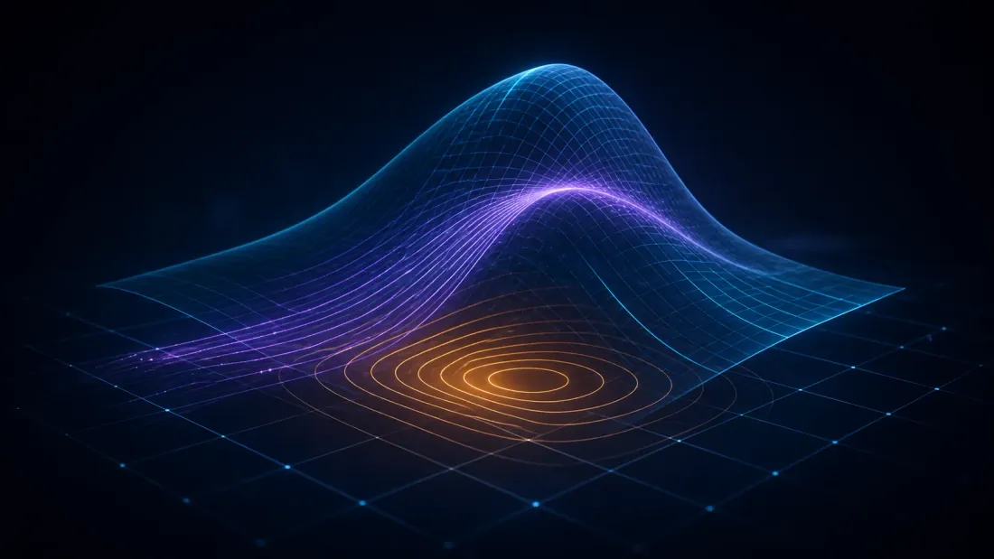
PDE Black-Scholes, терминальная выплата и лежащий в ее основе аргумент отсутствия арбитража разобраны в статье Формула Black-Scholes. Здесь мы предполагаем, что читатель с ними знаком, и сразу переходим к форме, на которой сеть действительно можно обучать.
Преобразование логарифма цены
Работать непосредственно с неудобно: область равна , а коэффициенты PDE зависят от переменной. Стандартное преобразование переводит уравнение в форму с постоянными коэффициентами:
Это уравнение конвекции - диффузии - реакции на . Переменные коэффициенты и исчезли, что важно для сети: невязка, масштаб которой зависит от , будет доминироваться дальней частью области, и оптимизатор станет тратить на нее весь ресурс.
Функция потерь PINN для Black-Scholes
Пусть - сеть. Выберем точек коллокации внутри области, точек на границах и точек в терминальный момент:
Каждая частная производная вычисляется через torch.autograd.grad с create_graph=True, поэтому при обратном распространении градиенты проходят через вычисление производной. Именно этот единственный флаг является главным приемом реализации.
Реализация на PyTorch

Параметры ниже ближе к крипторынку, чем к учебнику: и (примерно 30-дневный BTC-опцион), а не , , типичные для фондового стола. Короткий срок и высокая волатильность - режим, в котором излом выплаты наиболее резкий и PINN обучать сложнее всего, что и является целью примера.
import torch
import torch.nn as nn
import numpy as np

r = 0.05        # risk-free rate
sigma = 0.7     # volatility
K = 1.0         # strike (moneyness-normalized)
T = 0.08        # ~30 days
x_min, x_max = -1.0, 1.0  # log-price domain (S/K in [0.37, 2.72])

device = torch.device("cuda" if torch.cuda.is_available() else "cpu")


class BSPINN(nn.Module):
    """Physics-Informed Neural Network for Black-Scholes PDE."""

    def __init__(self, hidden_dim=128, num_layers=4):
        super().__init__()
        layers = [nn.Linear(2, hidden_dim), nn.Tanh()]
        for _ in range(num_layers - 1):
            layers += [nn.Linear(hidden_dim, hidden_dim), nn.Tanh()]
        layers.append(nn.Linear(hidden_dim, 1))
        self.net = nn.Sequential(*layers)

    def forward(self, x, t):
        inputs = torch.cat([x, t], dim=1)
        return self.net(inputs)


def compute_pde_residual(model, x, t):
    """Compute Black-Scholes PDE residual using autodiff."""
    x.requires_grad_(True)
    t.requires_grad_(True)
    u = model(x, t)

    grads = torch.autograd.grad(u, [x, t], grad_outputs=torch.ones_like(u),
                                create_graph=True)
    u_x, u_t = grads[0], grads[1]

    u_xx = torch.autograd.grad(u_x, x, grad_outputs=torch.ones_like(u_x),
                               create_graph=True)[0]

    residual = u_t + 0.5 * sigma**2 * u_xx + (r - 0.5 * sigma**2) * u_x - r * u
    return residual


def terminal_condition(x):
    """European call payoff: max(S - K, 0) = max(exp(x) - K, 0)."""
    return torch.relu(torch.exp(x) - K)


def train_pinn(epochs=10000, lr=1e-3, n_interior=5000, n_boundary=500, n_terminal=1000):
    model = BSPINN().to(device)
    optimizer = torch.optim.Adam(model.parameters(), lr=lr)
    scheduler = torch.optim.lr_scheduler.CosineAnnealingLR(optimizer, T_max=epochs)

    for epoch in range(epochs):
        optimizer.zero_grad()

        x_int = (torch.rand(n_interior, 1, device=device)
                 * (x_max - x_min) + x_min)
        t_int = torch.rand(n_interior, 1, device=device) * T

        residual = compute_pde_residual(model, x_int, t_int)
        loss_pde = (residual ** 2).mean()

        x_tc = (torch.rand(n_terminal, 1, device=device)
                * (x_max - x_min) + x_min)
        t_tc = torch.ones(n_terminal, 1, device=device) * T
        u_tc = model(x_tc, t_tc)
        loss_ic = ((u_tc - terminal_condition(x_tc)) ** 2).mean()

        t_bc = torch.rand(n_boundary, 1, device=device) * T

        x_lo = torch.full((n_boundary, 1), x_min, device=device)
        loss_bc_lo = (model(x_lo, t_bc) ** 2).mean()

        x_hi = torch.full((n_boundary, 1), x_max, device=device)
        target_hi = torch.exp(x_hi) - K * torch.exp(-r * (T - t_bc))
        loss_bc_hi = ((model(x_hi, t_bc) - target_hi) ** 2).mean()

        loss = loss_pde + 10.0 * loss_ic + loss_bc_lo + loss_bc_hi

        loss.backward()
        optimizer.step()
        scheduler.step()

        if epoch % 1000 == 0:
            print(f"Epoch {epoch:5d} | PDE: {loss_pde:.2e} | "
                  f"IC: {loss_ic:.2e} | BC: {loss_bc_lo + loss_bc_hi:.2e}")

    return model
Стоит отметить два структурных решения:
- Вес терминального условия. Выплата получает вес 10x, поскольку именно она определяет задачу. Без жесткого выполнения сеть может тривиально удовлетворить PDE, выдавая ноль везде: однородное PDE имеет бесконечно много решений, а терминальное условие выбирает одно из них.
- Повторная выборка точек коллокации на каждой эпохе. Точки выбираются заново на каждом шаге, что действует как стохастическая регуляризация невязки. Альтернатива - фиксированный набор точек - позволяет сети переобучиться на невязку именно в этих координатах.
Расширение до модели стохастической волатильности Heston

Black-Scholes оценивает цену при одной постоянной , и именно это предположение предназначено отвергать в прогнозировании волатильности GARCH(1,1). В Heston волатильность становится вторым стохастическим фактором - мгновенной дисперсией :
где - скорость возврата к среднему, - долгосрочная дисперсия, - волатильность волатильности, а .
Ценовое PDE двумерно по состоянию:
Именно здесь безсеточный метод начинает выглядеть привлекательно. Конечно-разностной схеме нужна сетка по - типичная сетка содержит узлов. Добавьте третий стохастический фактор, например стохастические ставки, и сетка становится непрактичной. Монте-Карло лучше масштабируется по размерности, но сходится медленно, особенно для греков.
Архитектура PINN для Heston
Сеть получает три входа , где . Смешанная производная - член, который усложняет схемы ADI, - требует всего еще одного вызова autograd.grad:
class HestonPINN(nn.Module):
    def __init__(self, hidden_dim=256, num_layers=5):
        super().__init__()
        layers = [nn.Linear(3, hidden_dim), nn.Tanh()]
        for _ in range(num_layers - 1):
            layers += [nn.Linear(hidden_dim, hidden_dim), nn.Tanh()]
        layers.append(nn.Linear(hidden_dim, 1))
        self.net = nn.Sequential(*layers)

    def forward(self, x, v, t):
        return self.net(torch.cat([x, v, t], dim=1))


def heston_pde_residual(model, x, v, t, kappa, theta, xi, rho, r):
    x.requires_grad_(True)
    v.requires_grad_(True)
    t.requires_grad_(True)
    u = model(x, v, t)

    u_x, u_v, u_t = torch.autograd.grad(
        u, [x, v, t], torch.ones_like(u), create_graph=True
    )
    u_xx = torch.autograd.grad(u_x, x, torch.ones_like(u_x), create_graph=True)[0]
    u_vv = torch.autograd.grad(u_v, v, torch.ones_like(u_v), create_graph=True)[0]
    u_xv = torch.autograd.grad(u_x, v, torch.ones_like(u_x), create_graph=True)[0]

    residual = (
        u_t
        + 0.5 * v * u_xx
        + rho * xi * v * u_xv
        + 0.5 * xi**2 * v * u_vv
        + (r - 0.5 * v) * u_x
        + kappa * (theta - v) * u_v
        - r * u
    )
    return residual
Обратите внимание: u_xv получается дифференцированием u_x по v, с повторным использованием графа, построенного первым вызовом. Симметрия смешанных производных означает, что дифференцирование u_v по x должно дать тот же тензор; в float32 это не будет выполнено точно, и разница является дешевым диагностическим тестом поведения графа.
Американские опционы и задачи со свободной границей
Американские опционы добавляют ограничение досрочного исполнения: стоимость никогда не должна быть ниже внутренней стоимости. PDE превращается в задачу со свободной границей, эквивалентную задаче линейного дополнительного условия (LCP):
где - оператор Black-Scholes, а - выплата. Есть два способа включить это в функцию потерь.
Штрафной метод
Заменим дополнительное условие гладким штрафом:
где велико (обычно от до ). Когда падает ниже внутренней стоимости, штраф возвращает ее вверх, и функция потерь PINN становится такой:
Архитектура не меняется, меняется только невязка. Цена - новый гиперпараметр с плохим компромиссом по обусловленности: слишком малое значение нарушает ограничение, слишком большое делает ландшафт функции потерь доминируемым штрафным членом.
Прямой подход со свободной границей
Обучайте совместно две сети: одну для цены , вторую для оптимальной границы исполнения . Функция потерь включает PDE в области продолжения, условие гладкого сопряжения на границе и выплату в области исполнения. Граница получается как самостоятельный выход, что и нужно для хеджирования книги американских опционов.
Модели скачкообразной диффузии с PINN

Модель Мертона добавляет скачки Пуассона к геометрическому броуновскому движению:
где - составной процесс Пуассона с интенсивностью и логнормальными размерами скачков. Оценка цены превращается в частичное интегро-дифференциальное уравнение (PIDE):
где - плотность множителя скачка.
Именно интеграл ломает конечно-разностный метод: он связывает каждую точку области со всеми другими, разрушая ленточную структуру, на которую опирается решатель. У PINN такой структуры нет, поэтому нечему разрушаться. Интеграл становится еще одним членом невязки, вычисляемым квадратурой в каждой точке коллокации, а поскольку сеть определена всюду, получается прямым проходом, а не интерполяцией:
def jump_integral(model, x, t, lam, mu_j, sigma_j, n_quad=32):
    """Approximate jump integral using Gauss-Hermite quadrature."""
    nodes, weights = np.polynomial.hermite.hermgauss(n_quad)
    nodes = torch.tensor(nodes, dtype=torch.float32, device=x.device)
    weights = torch.tensor(weights, dtype=torch.float32, device=x.device)

    y_nodes = mu_j + sigma_j * np.sqrt(2) * nodes
    integral = torch.zeros_like(x)

    for i in range(n_quad):
        x_shifted = x + y_nodes[i]
        v_shifted = model(x_shifted, t)
        integral += weights[i] * v_shifted

    integral *= 1.0 / np.sqrt(np.pi)
    return integral
Тогда невязка PIDE имеет вид:
где - квадратурное приближение. Цикл требует n_quad дополнительных прямых проходов на каждый шаг обучения, и все они попадают в граф autograd - настоящая цена скачков выражается в памяти, а не в математике.
Сравнение с традиционными методами

Структурные различия реальны и их можно сформулировать без бенчмарка:
| Критерий | Конечно-разностный метод | Монте-Карло | PINN |
|---|---|---|---|
| Нужна сетка/мэш | Да (структурированная сетка) | Нет | Нет (безсеточный метод) |
| Проклятие размерности | Сильное (>3D непрактично) | Слабое (сходимость ) | Слабое (емкость сети масштабируется) |
| Греки | Приближение конечными разностями | Траекторные/LR-оценки | Точные через autodiff |
| Повторное использование при смене параметров | Нужно решать заново | Нужно моделировать заново | Параметрический подход: обучить один раз |
| Американские опционы | SOR/PSOR для LCP | Регрессия Longstaff-Schwartz | Штраф или свободная граница |
| Границы ошибки | Да (порядок схемы) | Да (ЦПТ) | Нет - только эмпирическая функция потерь |
Строки производительности, которые обычно находились бы здесь - время обучения, задержка инференса, точность, - намеренно отсутствуют: их измерение является открытой работой, а не строкой таблицы.
Где PINN могут правдоподобно выиграть
Переоценка в реальном времени. После обучения вычисление является прямым проходом по батчу, поэтому вся книга переоценивается одним запуском ядра, а не одним решением на каждый набор параметров. Превзойдет ли это хорошо настроенный решатель Кранка - Николсона на реалистичных размерах книги, остается эмпирическим вопросом и здесь не измерено.
Модели высокой размерности. Стохастическая волатильность плюс стохастические ставки плюс скачки - это 4+ измерения, где конечно-разностные методы фактически погибают. PINN деградируют по размерности плавно, но обучение остается сложным.
Непрерывные греки. Сеть гладкая и дифференцируемая, поэтому Delta, Gamma, Theta и Vega получаются из той же механики autograd, что и невязка PDE: не нужны bump-and-revalue и шум конечных разностей. Это самое сильное утверждение статьи и одновременно то, для чего особенно нужна измеренная поверхность Gamma.
Параметрические решения. Если подать параметры модели (, , ) на вход сети, одна PINN сможет покрывать семейство моделей, а не только одну калибровку.
Где PINN испытывают трудности
Стоимость обучения. Для одного опциона с одним набором параметров конечно-разностное решение заканчивается раньше, чем PINN завершает первую тысячу эпох.
Нет границ ошибки. Конечно-разностные схемы с экстраполяцией Ричардсона достигают машинной точности при известном порядке сходимости. PINN сообщает значение функции потерь, которое не является границей ошибки. Варианты с учетом неопределенности (Bai et al., 2025) добавляют доверительные интервалы, но область еще молода.
Сложность оптимизации. Ландшафт функции потерь сильно не выпуклый, а веса между PDE, граничными и терминальными членами требуют настройки. Типичный сбой - сеть сводит невязку PDE почти к нулю, полностью игнорируя граничные условия: это вполне корректное решение неправильной задачи.
Воспроизводимость. Разные seed, распределения точек коллокации и настройки оптимизатора могут привести к существенно разным решениям. Ансамбли помогают, но увеличивают стоимость.
Последние два пункта особенно стоит превратить в графики, поскольку это сбои, с которыми столкнется любой, кто будет заново реализовывать этот подход.
Что еще нужно измерить
Честное состояние статьи таково: формулировки корректны и код запускается, но ничего здесь не прошло бенчмарк на железе или данных этого стола. Чтобы превратить вывод в результат, а не в вывод формул, нужно:
- Sup-норму и RMSE относительно замкнутой формулы Black-Scholes на сетке , для каждого seed, всего пять seed. Обычная цель из практики - совпадение до 4 и более знаков после запятой; важно проверить это при , и опубликовать seed, на которых результат ломается.
- Ошибку Delta и Gamma, а не только цены. Сеть, совпадающая по цене до четырех знаков, но дающая шумную , бесполезна для хеджирования, поэтому Gamma - критерий приемки.
- Время обучения по часам и задержку инференса одного опциона для книги из 10 000 опционов, в сравнении с решением Кранка - Николсона идентичной задачи на том же GPU.
- Намеренно воспроизвести режимы отказа. Уменьшить вес граничной функции потерь, пока сеть не начнет удовлетворять PDE и нарушать границу; запустить пять seed и построить разброс. Оба эксперимента дешевы и полезнее еще одной поверхности цены, которая выглядит корректно.
- Подогнать модель под реальные котировки BTC с Deribit или как минимум сохранить приведенные выше параметры, реалистичные для крипторынка, вместо возврата к , .
- Представить выбор архитектуры и оптимизатора как результаты, а не советы. Более широкая или более глубокая сеть,
tanhили ReLU (разрывная вторая производная ReLU должна заметно испортить невязку), сканирование , Adam затем L-BFGS или только Adam - все это эксперименты в одну строку. Пока они не выполнены, это пересказанные из литературы общие места, и статья не будет выдавать их за рекомендации.
Два структурных утверждения все же можно сделать без измерений, поскольку они являются свойствами формулировки, а не конкретного запуска: использовать координаты логарифма цены (PDE становится уравнением с постоянными коэффициентами, что является фактом алгебры) и дать терминальному условию больший вес, чем члену PDE (однородное PDE допускает нулевое решение, что является фактом задачи).
Что еще есть в этой области

Направления, о которых стоит знать, но которые здесь не тестировались:
- Адаптивная к невязке выборка коллокации - размещать точки там, где невязка велика: около страйка для Black-Scholes или около границы Феллера для Heston, а не равномерно. Реализация короткая:
def adaptive_resample(model, x_pool, t_pool, n_select):
    """Select collocation points with highest PDE residual."""
    with torch.no_grad():
        residuals = compute_pde_residual(model, x_pool, t_pool).abs()
    probs = residuals.squeeze() / residuals.sum()
    indices = torch.multinomial(probs, n_select, replacement=False)
    return x_pool[indices], t_pool[indices]
- Перенос обучения между страйками и сроками - дообучать модель от соседней пары вместо обучения с нуля, чтобы поддерживать библиотеку, покрывающую опционную цепочку.
- Physics-Informed Extreme Learning Machines - зафиксировать скрытые веса и обучать только выходной слой, сведя обучение к одному линейному решению. Выразительность ниже, но Black-Scholes имеет достаточно малую размерность, поэтому это может быть несущественно.
- Обучение операторов (DeepONet, FNO) - учить оператор решения, а не само решение, отображая , чтобы новым структурам выплаты не требовалось переобучение. См. DeepSVM.
Заключение

PINN не заменяют конечно-разностные методы или Монте-Карло. Для одного опциона малой размерности с одним набором параметров выигрывают конечные разности, и это даже не близкое сравнение. Аргумент в пользу PINN узок и конкретен: модели высокой размерности, где сетки перестают работать; параметрические решения, повторно используемые для книги; и греки, получаемые тем же проходом autodiff, что и цена.
Эта статья дает слой перевода: показывает, как смешанная производная Heston, свободная граница американского опциона и интеграл скачков Мертона превращаются в отдельные члены функции потерь. Но она пока не дает доказательств, что полученные сети достаточно точны для хеджирования. Это следующий этап, и пока он не выполнен, все выше следует воспринимать как вывод формул, а не как рекомендацию.
Ссылки и дополнительное чтение
- Raissi, M., Perdikaris, P., Karniadakis, G.E. (2019). Physics-informed neural networks: A deep learning framework for solving forward and inverse problems involving nonlinear partial differential equations. Journal of Computational Physics, 378, 686-707.
- Dhiman, A., Kaur, D. (2023). Physics Informed Neural Network for Option Pricing. arXiv preprint.
- Salvador, B. et al. (2023). Meshless methods for American option pricing through Physics-Informed Neural Networks. Engineering Analysis with Boundary Elements.
- Bai, G. et al. (2025). An uncertainty-aware physics-informed neural network solution for the Black-Scholes equation. arXiv preprint.
- Chen, Y. et al. (2025). Stochastic jump diffusion process informed neural networks for American option pricing under data scarcity. Applied Soft Computing.
- Benth, F.E. et al. (2025). DeepSVM: Learning Stochastic Volatility Models with Physics-Informed Deep Operator Networks. arXiv preprint.
- He, Y. et al. (2024). Finance-Informed Neural Network: Learning the Geometry of Option Pricing. arXiv preprint.
- MathWorks: Physics-Informed Neural Networks (PINNs) for Option Pricing. MATLAB Finance Blog, 2025.
- GitHub: BlackScholesPINN (PyTorch implementation).
- Raissi PINNs GitHub repository.
Авторы
Инженер торговых систем
Разработка торговых ботов с 2017 года: межбиржевой арбитраж (подключал до 30 бирж), парный арбитраж на коинтеграции между спотом и фьючерсами, скальпинг, фронтраннинг, торговля по новостям, сентиментный анализ, трендовые алгоритмы, а также алгоритмы управления и балансировки портфелей. Делает выставление ордеров до 1 мс, warehouse для big data, бэктестинг-движки, AI-агентов и интерфейсы для ботов (в т.ч. open-source profitmaker.cc). Стек: JS/TS, Python, Rust/Zig/Go, DevOps, backend, frontend, архитектура.
Читайте также

Нейронный оператор Фурье для финансового моделирования на основе PDE

Trade Classification When You Have No Side Flag: Tick, Quote, Lee-Ready, BVC