Hamiltonian Neural Networks: Does a Financial System Conserve Anything?

Ci sono due domande che puoi porre sulle reti neurali hamiltoniane e solo una di queste è interessante.
La domanda noiosa è "gli HNN sono stabili?" La risposta è sì, ed è un teorema, non un esperimento. Codifica le equazioni di Hamilton nell'architettura, integrale con uno schema simplettico e l'analisi degli errori all'indietro ti fornisce un errore energetico limitato su orizzonti esponenzialmente lunghi. Non c'entra nulla che riguardi la finanza. Non hai bisogno di un backtest per crederci.
La domanda interessante è quella che il risultato di stabilità presuppone silenziosamente: un vettore di stato finanziario ammette una quantità conservata? Un HNN non scopre se esiste. Si presume esiste e trova quello migliore in base a tale presupposto. Se i mercati non hanno conservato per le coordinate scelte, la rete convergerà comunque, produrrà comunque uno scalare uniforme, si integrerà comunque senza esplodere - e il tutto sarà un modello molto stabile del nulla.
Questo post costruisce il macchinario, poi passa la metà posteriore cercando di romperlo. L'affermazione in esame è ristretta e falsificabile: quella di un scelto coppia - diciamo prezzo logaritmico ed EMA dei rendimenti - è canonicamente coniugato, il che significa in realtà vale per alcuni . Questa è un'affermazione empirica, e la sezione teorica della bozza non dà motivo di crederci.
Meccanica Hamiltoniana: cosa c'è di realmente nuovo qui

Spazio delle fasi, sistemi dinamici, traiettorie e orbite sono già vocabolario su questo blog: vedere attrattori in algotrading per le definizioni e varietà complesse per la ricostruzione dello spazio delle fasi tramite l'incorporamento di Takens. Ciò che segue li presuppone.
La parte nuova è la struttura simplettica. La meccanica classica ha due formulazioni equivalenti. Newton dà . Hamilton dà una funzione scalare da cui seguono tutte le dinamiche:
Tre conseguenze contano e nessuna di esse è disponibile per un modello dinamico generico:
- si conserva lungo le traiettorie. Il sistema è confinato su una superficie ad energia costante — una varietà di dimensione inferiore all'interno dello spazio delle fasi. Questo è un vincolo rigido su dove può arrivare lo Stato, non una tendenza.
- La forma simplettica 2 viene conservato. Il volume dello spazio delle fasi è esattamente conservato (teorema di Liouville). Le traiettorie non possono convergere su un attrattore; il flusso è incomprimibile.
- Le dinamiche sono reversibili nel tempo. Esegui il flusso all'indietro e recuperi esattamente lo stato iniziale.
Vale la pena soffermarsi sul punto 2, perché è la tensione più acuta con tutto il resto di questo blog. Il teorema di Liouville afferma che un sistema hamiltoniano non ha attrattori. I flussi che preservano il volume non possono contrarsi su nulla. Se ritieni che i mercati abbiano una struttura attrattiva – e l’articolo sugli attrattori sostiene che sia così – allora sei già convinto che i mercati non siano hamiltoniani in senso stretto. Questo è un conflitto reale, non un tecnicismo, ed è il motivo per cui le estensioni dissipative riportate di seguito non sono un ripensamento.
Perché l'integratore è importante
Simula un sistema hamiltoniano con un integratore ingenuo (Eulero, RK4) e la traiettoria calcolata si allontana lentamente dalla superficie a energia costante. L'errore di troncamento locale è piccolo; l'errore geometrico è sistematico. Su orizzonti lunghi la simulazione diventa qualitativamente sbagliata: le orbite che dovrebbero chiudersi iniziano a spiraleggiare.
Le reti neurali standard hanno lo stesso difetto per una ragione più profonda. Uno stato di mappatura MLP sui derivati non ha alcun meccanismo per preservare nulla. Apprende adeguatamente le dinamiche locali e accumula errori che si aggravano.
La rivendicazione della conservazione, in breve

Questo blog ha già sostenuto che i mercati obbediscono a principi simili alla conservazione: Navier-Stokes for algotrading, parte 2 espone ampiamente il caso, dalla liquidità come massa fino alla gestione del rischio idrodinamico, e fornisce la corretta inquadratura econofisica. Allo stesso modo, l'ottimizzazione della media-varianza è già un sistema lagrangiano su questo blog: vedere Teoria del portafoglio di Markowitz per la forma quadratica vincolata e Esecuzione ottimale di Almgren-Chriss per il budget di rischio/ identificazione, dove svolge esattamente il ruolo di un momento coniugato.
Niente di tutto ciò viene derivato qui, perché la mossa interessante è diversa. Questi articoli utilizzano la conservazione come una metafora che motiva un modello. Un HNN trasforma la conservazione in un vincolo architettonico che il modello non può violare anche se i dati lo implorano. Quella differenza – analogia morbida rispetto a struttura dura – è l’intero contenuto di ciò che segue, e taglia in entrambe le direzioni: un vincolo che i dati non soddisfano non è a priori, è un bug.
Architettura HNN: conservazione strutturale e conservazione penalizzata
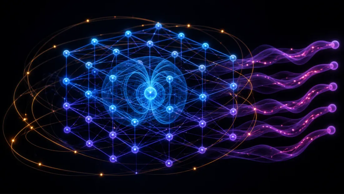
Il meccanismo generale basato sulla fisica - prendere le derivate autogradanti dell'output della rete rispetto ai suoi input, formare un residuo fisico, minimizzarlo - è già dimostrato nel Navier-Stokes PINN, il cui physics_loss costruisce u_t, u_x, u_xx tramite autograd.grad e eleva al quadrato il residuo. L'HNN utilizza lo stesso meccanismo con una modifica, e la modifica è il punto centrale.
Un PINN penalizza le violazioni di una legge fisica. Il residuo è un termine di perdita con un peso; l'ottimizzatore lo scambia con l'adattamento dei dati. Riduci il peso o fornisci dati contrastanti e la rete violerà felicemente la legge. La conservazione è una preferenza.
Un HNN rende la conservazione strutturale. Non apprende il campo vettoriale , che non è vincolato e non conserva nulla. Impara uno scalare e deriva entrambe le componenti del campo vettoriale da un singolo gradiente:
Poiché entrambe le derivate provengono da un potenziale scalare, il campo risultante è un gradiente simplettico per costruzione. , in modo identico, per ogni impostazione dei parametri — compresa una rete inizializzata in modo casuale e completamente non addestrata. Non c'è peso da sintonizzare. La conservazione è un'identità algebrica della parametrizzazione, non un termine nell'obiettivo.
Questa è una garanzia molto più forte di quella offerta da un PINN e viene fornita con una modalità di errore molto più nitida. La perdita confronta i derivati derivati con i dati osservati:
Se l'osservato Il campo non è un gradiente simplettico di qualcosa – se ha un ricciolo la parametrizzazione non può rappresentarlo – la perdita semplicemente non può raggiungere lo zero. Il pavimento residuo non è un errore di ottimizzazione. È una misura di quanto i dati sono lontani dall'ammettere un hamiltoniano. Quel numero è l'output più utile dell'intera architettura, ed è il numero attorno al quale è organizzato il resto di questo post.
La rete in sé è insignificante: un MLP da attraverso due strati tanh di larghezza 200 ad un output scalare.
Coordinate
Per le applicazioni finanziarie, è una posizione generalizzata (prezzi logaritmici, pesi del portafoglio, esposizioni fattoriali) e uno slancio generalizzato (tassi di cambiamento, indicatori di slancio, variabili di flusso). è quindi qualunque invariante che la rete riesca a trovare: forse la capitalizzazione di mercato totale, forse una misura di rischio, forse una quantità astratta senza lettura economica, forse niente.
La scelta dell'abbinamento non è innocente, ed è questa la lacuna nella presentazione standard. Niente riguardo" = prezzo logaritmico, = EMA dei rendimenti" stabilisce che questi sono coniugati. La coniugazione è una relazione strutturale specifica — deve essere lo slancio canonicamente abbinato , tale che vale per alcuni . Affermarlo e testarlo sono attività diverse, e la letteratura che adatta gli HNN alla finanza si occupa principalmente della prima.
| (posizioni) | (momento) |
|---|---|
| Prezzi dei tronchi | EMA dei rendimenti |
| Pesi del portafoglio | Tassi di variazione del peso |
Integratori simplettici
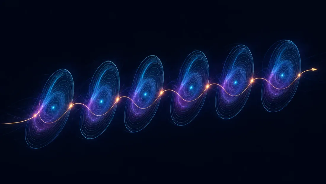
Apprendimento è metà del problema. La generazione di traiettorie richiede l'integrazione delle equazioni di Hamilton e l'integratore può distruggere ciò che l'architettura garantisce.
Integratori simplettici preservare esattamente. Il volume dello spazio delle fasi si conserva, oscilla attorno al suo vero valore con errore limitato anziché andare alla deriva secolare, e le orbite rimangono qualitativamente corrette. RK4 fornisce un errore per passaggio più piccolo e nessuna di queste proprietà.
Lo schema simplettico più semplice è Stormer-Verlet (leapfrog):
Per separabile questi sono aggiornamenti espliciti. Gli Hamiltoniani finanziari sono generalmente non separabili – le dinamiche del momentum dipendono dai prezzi e viceversa – quindi il caso generale necessita di passaggi impliciti, metodi di ordine superiore (Yoshida, Forest-Ruth) o il percorso SympNets di seguito.
Tong et al. (2020) hanno dimostrato che la composizione dei passaggi leapfrog come strati di rete produce architetture che sono simplettiche per costruzione: ogni livello è un passaggio di integrazione, la profondità equivale al conteggio dei passaggi e la mappa appresa preserva esattamente la struttura simplettica.
Garanzie di stabilità: reali e non pertinenti

Le proprietà di stabilità derivano dai teoremi, ed è proprio per questo che non dimostrano nulla sui mercati.
Analisi dell'errore all'indietro. Un integratore simplettico applicato a risolve esattamente un hamiltoniano vicino . La traiettoria calcolata è la traiettoria esatta di un sistema leggermente perturbato e la teoria KAM limita l'errore energetico su tempi esponenzialmente lunghi.
Stabilità di Lyapunov. Se ha un minimo in equilibrio, è essa stessa una funzione di Lyapunov che dimostra che l'equilibrio è stabile. Non è richiesta alcuna analisi separata.
Entrambi i risultati sono condizionali essere l'oggetto giusto. Ti dicono che la simulazione del sistema appreso è fedele; non dicono nulla sul fatto che il sistema appreso sia il mercato. Uno perfettamente conservato montato su un pavimento residuo di 0,9 è una simulazione stabile di un manufatto.
| Immobile | Standard NN + RK4 | HNN + simplettico |
|---|---|---|
| Deriva energetica oltre 1000 passi | secolare, accumula | limitato, oscillatorio |
| Reversibilità temporale | no | sì |
| Volume dello spazio delle fasi | non conservato | esattamente conservato |
| Attrattori rappresentabili | sì | no (Liouville) |
| Invariante interpretabile | nessuno |
Implementazione

Modulo HNN principale
import torch
import torch.nn as nn

class HamiltonianNN(nn.Module):
    """Learns a scalar H(q, p); derives dynamics via Hamilton's equations."""
    def __init__(self, input_dim: int, hidden_dim: int = 200):
        super().__init__()
        self.net = nn.Sequential(
            nn.Linear(input_dim, hidden_dim), nn.Tanh(),
            nn.Linear(hidden_dim, hidden_dim), nn.Tanh(),
            nn.Linear(hidden_dim, 1),
        )

    def hamiltonian(self, q: torch.Tensor, p: torch.Tensor) -> torch.Tensor:
        return self.net(torch.cat([q, p], dim=-1))

    def time_derivative(self, q: torch.Tensor, p: torch.Tensor):
        q = q.requires_grad_(True)
        p = p.requires_grad_(True)
        H = self.hamiltonian(q, p)
        dH_dq, dH_dp = torch.autograd.grad(H.sum(), [q, p], create_graph=True)
        return dH_dp, -dH_dq          # dq/dt, dp/dt
Integratore simplettico Leapfrog
class LeapfrogIntegrator:
    """Stormer-Verlet integrator. Preserves the symplectic structure."""
    def __init__(self, hnn: HamiltonianNN, dt: float = 0.01):
        self.hnn, self.dt = hnn, dt

    def step(self, q: torch.Tensor, p: torch.Tensor):
        _, dp_dt = self.hnn.time_derivative(q, p)
        p_half = p + 0.5 * self.dt * dp_dt

        dq_dt, _ = self.hnn.time_derivative(q, p_half)
        q_new = q + self.dt * dq_dt

        _, dp_dt = self.hnn.time_derivative(q_new, p_half)
        return q_new, p_half + 0.5 * self.dt * dp_dt

    def integrate(self, q0, p0, n_steps: int):
        traj_q, traj_p, q, p = [q0], [p0], q0, p0
        for _ in range(n_steps):
            q, p = self.step(q, p)
            traj_q.append(q); traj_p.append(p)
        return torch.stack(traj_q), torch.stack(traj_p)
Coordinate dello spazio delle fasi
Prezzi logaritmici, rendimenti differenziati, slancio EMA e volatilità variabile sono la struttura standard di questo blog: la pipeline del modello di diffusione e varietà complesse lo forniscono entrambi. Le uniche due righe che contano qui sono quelle che definiscono la coppia coniugata:
q = np.log(prices)[w:-1]                          # generalised position
p = ewma(np.diff(np.log(prices), axis=0), w)[w-1:-1]   # generalised momentum
Tutto a valle: differenza finita , , l'allineamento della lunghezza, il ciclo di addestramento che confronta i derivati derivati con quelli osservati con Adam - è meccanico.
Verifica della conservazione
def measure_conservation(hnn, integrator, q0, p0, n_steps=1000):
    """Energy drift along an integrated trajectory."""
    with torch.no_grad():
        traj_q, traj_p = integrator.integrate(q0, p0, n_steps)
        energies = torch.stack([
            hnn.hamiltonian(traj_q[i], traj_p[i]) for i in range(n_steps + 1)
        ]).squeeze().numpy()

    return {
        "H_initial": energies[0],
        "H_final": energies[-1],
        "drift": energies[-1] - energies[0],
        "oscillation": energies.std(),
        "relative_error": abs(energies[-1] - energies[0]) / abs(energies[0]),
    }
Nota cosa questa funzione non testa. Misura se l'integratore preserva - cosa che, per teorema, lo farà o no significa qualsiasi cosa. La conservazione nel campione di un hamiltoniano appreso non è una prova. Il test che conta è diverso.
Il test di falsificazione
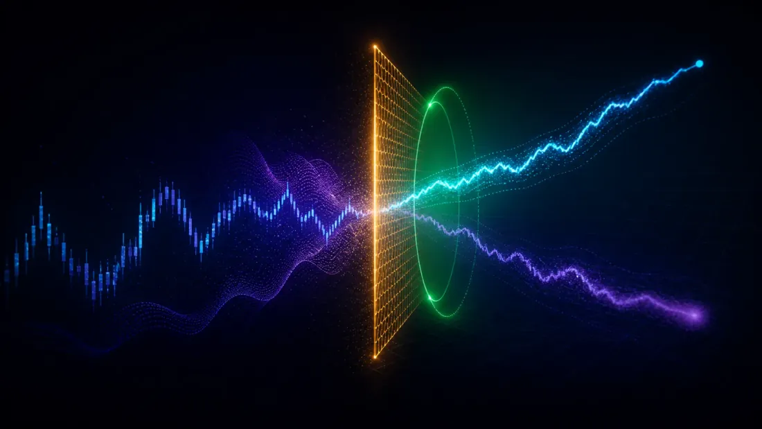
L’esperimento onesto è composto da tre parti ed è progettato in modo tale che un risultato negativo sia informativo anziché imbarazzante.
1. Piano residuo. Adatta sui dati reali e riportare la perdita convergente, non la conservazione. Una parametrizzazione a gradiente simplettico non può rappresentare un campo vettoriale con arricciatura; il pavimento misura la componente non hamiltoniana della dinamica osservata. Adattare un MLP non vincolato sugli stessi dati di riferimento: non ha restrizioni strutturali, quindi il divario tra i due piani è il costo dell'ipotesi hamiltoniana, espresso nelle unità di perdita del problema.
2. Conservazione dei campioni fuori campione. Adattare su una finestra, quindi valutare lungo la traiettoria osservata fuori campione: il percorso del prezzo reale, non integrato. Se è veramente canonico, rimane più o meno costante lungo i dati che non ha mai visto. Se esce dal campione, la quantità conservata era un artefatto nel campione e la garanzia dell'architettura non funziona.
3. Ablazione coordinata. Questa è la parte richiesta dalla sezione teorica e nessuna presentazione degli HNN finanziari sembra funzionare. Nulla stabilisce che il prezzo logaritmico e l'EMA dei rendimenti siano coniugati; si afferma. Quindi testa gli abbinamenti uno contro l’altro – (prezzo logaritmico, rendimenti EMA), (prezzo logaritmico, rendimenti grezzi), (pesi del portafoglio, tassi di variazione del peso) – e classificali in base al fuori campione stabilità. Contro un surrogato del controllo con rendimenti mescolati: distruggere la struttura temporale, mantenere la distribuzione marginale, riadattarla. Se il surrogato produce risultati comparabili stabilità, la “quantità conservata” è una proprietà della parametrizzazione più che del mercato.
Il mio precedente, dichiarato prima del fatto in modo che possa essere verificato rispetto al risultato: questo fallisce. Il ragionamento è nel primer qui sopra: il teorema di Liouville vieta gli attrattori, i mercati sembrano avere una struttura attrattiva ed entrambe le vie di fuga sottostanti sono ammissioni che il rigoroso presupposto hamiltoniano non regge. Se il pavimento residuo è alto e fuori campione è instabile in ogni abbinamento, ovvero un negativo misurato pulito su un precedente basato sulla fisica, e questo blog ha pubblicato quelli precedenti (the onesto negativo, deflated Sharpe). Un negativo misurato su una teoria elegante vale più di un tutorial non testato.
Se la conservazione fallisce: estensioni dissipative

I mercati reali perdono. I costi di transazione, lo slittamento e il decadimento dell'informazione tolgono energia al sistema e la conservano rigorosamente non può rappresentarlo. Esistono due rilassamenti di principio, ed entrambi dovrebbero essere letti come concessioni che l'assunzione fosse troppo forte, non come perfezionamenti:
- Hamiltoniana conforme: modello con un tasso di dissipazione appreso . L'entità dell'adattamento è di per sé una misura: quanto il sistema si trova lontano dal conservatore.
- Port-Hamiltoniano: , con la matrice simplettica, la matrice di dissipazione, e forzanti esterne (notizie, flussi). Qui relativo a quantifica direttamente la partenza.
Entrambi ripristinano la capacità di rappresentare attrattori, a scapito della garanzia di errore limitato che ha motivato l'architettura. Questo è il mestiere, detto chiaramente: puoi avere Liouville o puoi avere la dissipazione, e i mercati sembrano volere la seconda.
Problemi aperti correlati: gli hamiltoniani finanziari non sono separabili (richiedono passaggi simplettici impliciti o di ordine superiore, o SympNet imparando direttamente le mappe simplettiche) e i mercati operano su più scale temporali rispetto a una singola è improbabile che possa catturare: hamiltoniani gerarchici per dinamiche veloci e lente, o un trattamento adiabatico di variabili lente come parametri di una scala veloce .
Conclusione

Il macchinario funziona. Impara uno scalare , deriva il campo vettoriale dal suo gradiente, lo integra in modo simplettico e ottieni la conservazione come identità algebrica, errore limitato su migliaia di passaggi, reversibilità temporale esatta e una funzione di Lyapunov gratuitamente. Ognuna di queste affermazioni è un teorema e nessuna di esse richiede convalida.
Ciò che richiede la convalida è la premessa. Gli HNN non verificano se esiste una quantità conservata: la assumono e ottimizzano in base al presupposto, convergendo a prescindere in un modello fluido, stabile e ben educato. Il pavimento residuo e il fuori campione stabilità sono gli unici due numeri che distinguono “il mercato conserva qualcosa” da “la parametrizzazione produce sempre qualcosa”.
Quindi la domanda con cui termina questo post non è se gli HNN siano stabili. La questione è se l'eleganza sopravvive al contatto con BTCUSDT e finché questi numeri non saranno pubblicati, l'atteggiamento corretto nei confronti di ogni affermazione di conservazione nell'apprendimento automatico finanziario, incluso questo, è che non sia stata testata.
Riferimenti
- Greydanus, S., Dzamba, M., & Sprague, J. (2019). Reti Neurali Hamiltoniane. NeurIPS 2019.
- Tong, Y., Xiong, S., He, X., Pan, G. e Zhu, B. (2020). Reti hamiltoniane profonde basate su integratori simplettici. arXiv prestampa.
- Baaquie, BE (2000). Hamiltoniano nei mercati finanziari. arXiv prestampa.
- Cotler, J. e Rezchikov, S. (2023). Simulazione hamiltoniana efficiente per risolvere la dinamica dei prezzi delle opzioni. Ricerca sulla revisione fisica.
- Gonon, P. & Ortega, J.-P. (2009). Mercati azionari e dinamica quantistica. arXiv prestampa.
- Greydanus, S. (2019). Reti neurali hamiltoniane – post sul blog.
- Santos, C. et al. (2022). Reti neurali del momento simplettico. PMLR.
Autori
Trading-systems engineer
Trading-systems engineer building bots since 2017: cross-exchange arbitrage (connected up to 30 venues), cointegration-based pairs arbitrage across spot and futures, scalping, news and sentiment-driven strategies, trend algorithms, and portfolio management and balancing algorithms. Also builds sub-millisecond order execution, big-data warehouses, backtesting engines, AI agents, and trading interfaces (incl. open-source profitmaker.cc). Stack: JS/TS, Python, Rust/Zig/Go, DevOps, backend, frontend, architecture.
Leggi di Più

Neural ODEs: Does Continuous Time Beat a Delta-Time Feature?

Trade Classification When You Have No Side Flag: Tick, Quote, Lee-Ready, BVC