Stratégies LP Uniswap v3 et couverture
Une position passive Uniswap v3 est un ensemble d’ordres limités au repos que vous ne pouvez pas annuler. Un portefeuille actif – plage choisie, recentrée sur un calendrier, couvert sur un perp – est un livre de tenue de marché, et il doit être géré comme tel. Ce recadrage change chaque décision. Un teneur de marché évalue les cotations à partir d’une prévision de volatilité, et non d’une intuition. Un teneur de marché traite chaque recotation comme un coût et non comme un réflexe. Un teneur de marché connaît à tout moment son delta de stock et décide délibérément de le porter ou de le couvrir. Et un teneur de marché sait que certaines de ses contreparties sont plus rapides et mieux informées, et il intègre cela dans ses prix.
L'article sur la liquidité concentrée a construit les primitives : ticks, liquidité , les formules de montant symbolique, feeGrowthInside, et le fait qu'une position LP est un gain à faible volatilité dont le coût de fonctionnement est la perte par rapport au rééquilibrage (LVR). Cette pièce est le manuel de l'opérateur au-dessus de cette fondation. Nous évaluons la fourchette à partir d'une prévision de variance, définissons la décision de rééquilibrage comme une transaction explicite entre gain de frais attendu et coût réalisé, déduisons le delta de la position directement à partir de la fonction de valeur et le neutralisons avec des contrats à terme perpétuels, considérons la liquidité juste à temps (JIT) comme le cas extrême du LPing actif, et terminons par la manière dont un backtest honnête en chaîne de tout cela peut vous mentir. Tout au long, le modèle mental est Avellaneda-Stoikov avec deux modifications brutales : vos cotations sont inscrites dans un registre public avant d'être remplies, et chaque nouvelle cotation coûte de l'essence.
Largeur de plage à partir d'une prévision de volatilité
Le paramètre le plus important d’un LP actif est la largeur de la range, et il s’agit d’un pari purement volatile. Trop large et vous diluez votre liquidité sur des ticks qui se négocient rarement, gagnant des frais au taux anémique d'un pool v2. Trop étroit et vous concentrez magnifiquement la profondeur - jusqu'à ce que le prix sorte de votre fourchette, vous passez à 100 % dans l'actif perdant et vous ne gagnez rien jusqu'à ce que vous rééquilibriez (cristallisant la perte de divergence en cours de route). La largeur optimale est celle qui maintient le prix à l'intérieur de la fourchette suffisamment souvent pour que le taux de frais concentré fasse plus que payer le LVR amplifié par la concentration. Il s’agit d’une déclaration sur la distribution des rendements futurs, vous la dimensionnez donc à partir d’une prévision de cette distribution.
Modèle de prix des logs sur un horizon de détention comme environ , avec la volatilité par période. Un symétrique -la plage sigma dans le prix du journal est
donc et . Choisir c'est choisir la probabilité de rester à portée : maintient le prix à l'intérieur pendant environ 68 % des horizons, pour ~95%. Plus large négocie le taux des frais en fonction du temps compris dans la plage, et le point idéal dépend du niveau de frais et du régime de vol – qui est exactement la quantité qu'un teneur de marché prévoit plutôt que devine.
La traduction en paramètres en chaîne est une ligne, car les ticks sont le prix du journal. Depuis , l'indice de tick est , et , donc la demi-largeur en graduations est d'environ . Accrochez-vous à l'espacement des graduations du pool et vous avez vos limites :
import numpy as np

TICK = np.log(1.0001)   # ≈ 1.0000e-4, one tick in log-price

def range_from_vol(price, sigma_per_day, horizon_days, k=1.0, spacing=10):
    """Symmetric k-sigma range -> tick bounds for a v3 position.
    `price` is the RAW pool price (token1/token0, base units)."""
    sig_h = sigma_per_day * np.sqrt(horizon_days)     # vol over the horizon
    i0 = round(np.log(price) / TICK)                  # current tick
    half = round(k * sig_h / TICK)                    # half-width in ticks
    lower =  ((i0 - half) // spacing) * spacing        # floor to spacing
    upper = -(-(i0 + half) // spacing) * spacing       # ceil  to spacing
    return lower, upper, np.exp(lower*TICK), np.exp(upper*TICK)
Un numéro travaillé corrige l'intuition. Prenez l'ETH avec un vol quotidien prévu de 4%, un horizon de recentrage d'une semaine ( jours), et . Alors , donc la plage s'étend , c'est-à-dire à peu près — à propos d'un groupe, ou les tiques se sont alignées sur l'espacement. La largeur est linéaire dans la prévision de volume (au premier ordre dans l'espace log), c'est là tout l'intérêt : votre concentration de liquidité doit respirer avec celle du marché, et non rester statique "± 10 % parce que cela vous semblait correct le mois dernier". Variez les deux boutons – le régime et la confiance - et la bande évolue de la même manière que le spread coté d'un teneur de marché évolue :
| Prévisions quotidiennes | Régime | demi-largeur | demi-largeur | Env. coches () |
|---|---|---|---|---|
| 2% | calme | ±5,3% | ±10,6% | ±529 |
| 4% | normale | ±10,6% | ±21,2% | ±1058 |
| 6% | élevé | ±15,9% | ±31,8% | ±1587 |
| 8% | stressé | ±21,2% | ±42,3% | ±2116 |
Lisez le tableau comme une politique de citation et non comme une recherche. Une bande plus étroite génère un taux de frais par dollar plus élevé lorsqu'elle est dans la plage (plus de profondeur par tick), mais sort de la plage plus tôt et se recentre plus souvent ; une bande plus large est le contraire. Le multiplicateur de liquidité concentrée est le levier – un le groupe cite environ un ordre de grandeur de plus de profondeur par tick qu'une position v2 complète et gagne des frais à ce multiple pendant qu'il est dans la plage - mais c'est aussi ce même multiple plus exposé au LVR. La largeur de plage est l'endroit où vous choisissez votre point sur la frontière du taux de frais par rapport au temps passé dans la plage, et la prévision de volume est ce qui vous indique où se situe cette frontière aujourd'hui.
Une contrainte limite l’extrémité serrée : l’espacement des ticks. Vos limites doivent s'aligner sur l'espacement du niveau de frais, de sorte que la plage minimale que vous pouvez exprimer est définie par le pool que vous avez choisi : environ ±10 pb sur le niveau de 0,05 % (espacement 10), ±60 pb sur le niveau de 0,30 % (espacement 60), ±2 % sur le niveau de 1 % (espacement 200). Cela associe deux décisions qui semblent indépendantes : la sélection du niveau de frais est une sélection de plage-résolution. Une paire stable dont la prévision de volume veut une bande de ±0,3 % ne peut la réaliser qu'au niveau de 0,05 % ; essayez-le au niveau de 1% et la grille de cocher vous oblige au moins huit fois trop large, diluant la concentration même pour laquelle vous payiez les frais les plus élevés. Faites correspondre la granularité du niveau à la largeur demandée par vos prévisions, et non l'inverse.

Où est-ce que venir de? La volatilité réalisée sur une fenêtre suiveuse est la réponse grossière et elle est très rétrospective : elle vous indique la fourchette que vous auriez dû définir la semaine dernière. Le bon outil est un modèle à variance conditionnelle qui réagit au régime actuel : une prévision GARCH(1,1) agrégée à l'horizon, telle que développée dans GARCH Volatility Forecasting for Crypto. GARCH vous offre et, en itérant la récursion, un -variance pas en avant dont la racine carrée est la tu veux. L'effet de levier de la crypto - le vol saute davantage lors des mouvements vers le bas - plaide en faveur d'une variante asymétrique et du même [machinerie de ciblage du vol] (/blog/volatility-targeting-garch-strategy) qui redimensionne une position directionnelle en redimensionne une plage LP de : sens inverse, prévision identique. Introduisez cette série dans range_from_vol à chaque recentrage et la concentration de la position suit automatiquement les prévisions. Ce qui soulève la question suivante sur laquelle se pose cet article : à quelle fréquence devriez-vous vous recentrer ?
Rééquilibrage : l'échange de frais-gains par rapport au coût réalisé
Le rééquilibrage excessif est le principal destructeur des rendements des LP au détail, et c'est un tueur subtil car chaque individu recentré se sent responsable. Le prix a dérivé vers le bord de votre fourchette, vous vous êtes donc recentré pour « rester actif ». Mais un recentrage v3 n'est pas une recotation gratuite sur un CEX. Il s’agit de trois coûts superposés :
- Gas — brûlez l'ancienne position, créez la nouvelle et (généralement) un échange pour rééquilibrer l'inventaire. Sur le réseau principal, cela représente un coût fixe par cycle non trivial, brutal pour les petites positions.
- Coût de swap — pour recentrer, vous devez échanger votre inventaire déséquilibré vers le ratio de la nouvelle fourchette, en payant les frais de swap et l'impact du prix sur cette transaction.
- LVR cristallisé — c'est le LVR invisible. Alors que le prix variait, la position a accumulé une perte de divergence sur papier. Maintenir un prix aller-retour permettrait d'en récupérer une grande partie (vous conservez les frais, restituez l'évolution des stocks). Le recentrage réalise cette perte : vous vendez l'actif dans lequel vous êtes maintenant lourd, à un prix déprimé, et vous le réinitialisez. Chaque recentr convertit le LVR papier en LVR réservé.
La décision de rééquilibrage n’est donc pas « suis-je proche du bord ? » mais le calcul de requotation d'un teneur de marché : l'augmentation future des frais attendue à partir d'une position mieux centrée dépasse-t-elle le coût réalisé pour y arriver ? Il s'agit structurellement du problème de contrôle des coûts de transaction - la politique optimale est une bande de non-rééquilibrage autour du centre, pas un fil-piège. À l’intérieur du groupe, vous laissez les stocks dériver et continuez à percevoir des frais ; vous n’agissez que lorsque le bénéfice attendu compense le coût.
def should_rebalance(pos, price, fee_apr, sigma, gas_usd, swap_bps):
    """Rebalance only if expected fee uplift beats the realized recenter cost."""
    V = pos.value(price)
    recenter_cost = (gas_usd
                     + swap_bps * 1e-4 * pos.inventory_to_swap(price)  # fee+impact
                     + pos.crystallized_lvr(price))                    # the hidden one
    tau = pos.expected_time_in_range(price, sigma)   # horizon until next recenter
    fee_uplift = (pos.fee_rate_centered(price) - pos.fee_rate_now(price)) \
                 * fee_apr * V * tau
    return fee_uplift > recenter_cost
Une décision de rééquilibrage avec des chiffres
Rendez-le concret. Supposons que vous déteniez une position de 50 000 r^{\text{now}} = 8%r^{\text{centered}} = 30%\mathbb{E}[\tau] \approx 5= 0.0137$ des années avant de vous recentrer à nouveau. L'augmentation brute est
En contrepartie, le coût du recentrage : 25 passe à 5 pb de frais plus impact pour 10 . Coût total réalisé . Depuis , vous vous recentrez – mais notez à quel point il est proche et comment un pic de gaz de 5 avec les mêmes pourcentages : la hausse tombe à 15 , et l'échange ne vaut jamais la peine d'être fait. Le terme de majoration des frais évolue avec le notionnel ; le terme gaz ne le fait pas. Cette asymétrie unique est la raison pour laquelle les petits LP du réseau principal devraient soit fonctionner sur une plage large et rarement touchée, soit rester à l'écart.
Seuil versus périodique
Deux régimes sortent de cette inégalité, et ils constituent la réponse honnête à la question « basé sur un seuil ou périodique ». Le rééquilibrage de seuil (bande) – qui agit lorsque le prix sort d'une bande de tolérance – est la forme théoriquement correcte, car elle conditionne l'état qui compte réellement. Rééquilibrage périodique — recentrer tous les des blocs ou des heures indépendamment - est une approximation grossière qui n'est défendable que parce qu'elle est plus simple à exécuter et plus facile à raisonner ; sa pathologie se recentre lors d'un clapot qui aurait inversé la moyenne gratuitement, en payant de l'essence et en cristallisant le LVR pour un aller-retour que vous auriez gagné en ne faisant rien. Empiriquement, plus votre niveau de frais est large et plus le gaz est élevé, plus votre bande devrait être large et plus vos rééquilibrages sont rares – un pool de 1 % recentré quotidiennement allume presque toujours l’argent en feu. Le corollaire inconfortable : pour de nombreuses petites positions sur le réseau principal, le terme d'augmentation des frais n'efface jamais le terme de gaz, et le nombre correct de rééquilibrages est zéro – définissez une large plage une fois et laissez-la, ou ne faites pas de LP du tout.
C’est aussi pourquoi le lieu compte autant que la stratégie. L’ensemble des inégalités est dominé par le terme gaz sur le réseau principal Ethereum, où un cycle de rééquilibrage coûte de l’argent réel ; sur une L2 (Arbitrum, Base, Optimisme) le même cycle coûte des centimes, donc s'effondre, la bande qui la dégage se rétrécit et le LPing actif à courte portée avec un recentrage fréquent devient viable exactement pour les petites positions qui ne pourraient jamais se le permettre sur L1. Ce n’est pas une note de bas de page – c’est pourquoi les stratégies LP actives sérieuses ont largement migré vers les L2, et pourquoi « à quelle fréquence rééquilibrer » a une réponse différente sur chaque chaîne. Cependant, les conditions du LVR et des coûts de swap ne diminuent pas avec le gaz, de sorte que le gaz bon marché abaisse autant l'obstacle au rééquilibrage excessif qu'à un rééquilibrage raisonnable ; la discipline de l'inégalité compte plus là où le gaz cesse de l'appliquer à votre place.
Il existe une troisième option qui évite complètement le recentrage : la plage unilatérale. Au lieu d'une bande symétrique que vous faites glisser pour suivre le prix, placez une fourchette asymétrique qui exprime un point de vue : liquidité uniquement en dessous du point si vous êtes heureux d'accumuler l'actif à la baisse, uniquement au-dessus si vous souhaitez le distribuer à la hausse. Il s'agit du cas d'utilisation des ordres limités en chaîne, et il transforme un « rééquilibrage » en une « recharge » : lorsqu'une fourchette unilatérale se remplit complètement (le prix la dépasse), vous avez exécuté votre achat ou votre vente prévu à un prix moyen majoré des frais, et la décision est de savoir s'il faut se réarmer, pas s'il faut poursuivre. Pour les mandats d'accumulation et de distribution, il domine le recentrage symétrique, car le mouvement de stock que vous combattriez avec une couverture est la position que vous souhaitiez réellement.
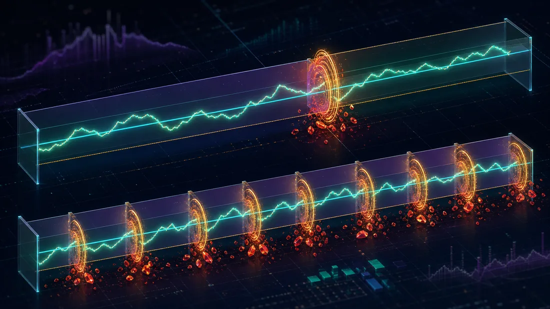
La connexion au LVR mérite d'être soulignée, car elle relie toute cette série : la somme de vos pertes de recentrage réalisées sur la durée de vie d'une position, correctement comparée, converge vers le LVR que l'analyse IL/LVR prédit à partir de la variance réalisée de la trajectoire des prix. Le rééquilibrage n'évite pas le LVR ; il choisit quand le payer et dans quelle devise. Rééquilibrez trop souvent et vous payez également des frais d'essence et d'échange en plus du LVR que vous alliez payer de toute façon. C’est pourquoi le sur-rééquilibrage domine les modes de défaillance : il s’agit du LVR plus une taxe auto-infligée.
Couverture delta du LP avec des contrats à terme perpétuels
Si la largeur de la range est votre pari de volume et la bande de rééquilibrage est votre politique d'inventaire, la couverture delta est la façon dont vous séparez les deux afin que vous exécutiez un livre de tenue de marché (vol court, collectez le spread) et non un livre directionnel (ETH long ou court par accident). Pour couvrir, vous avez besoin du delta de la position, et la beauté de la v3 est qu'il sort directement de la fonction de valeur sans chiffres.
La valeur d'une position dans la fourchette, en unités de token1 (le numéraire, par exemple USDC), est l'expression dérivée dans la pièce à liquidité concentrée :
Se différencier par le prix de l'actif risqué (token0, par exemple ETH) :
Le delta de la position est égal au montant de token0 que la position détient actuellement. Ce n'est pas une coïncidence et cela vaut la peine de s'arrêter sur : , donc , et l'invariant AMM rend la valeur commerciale marginale sur la courbe neutre au prix actuel, c'est-à-dire . Les deux termes finaux s’annulent et le delta correspond uniquement à l’inventaire ETH. Un LP est long sur l'actif risqué exactement pour le montant actuellement dans la position – un nombre qui diminue à mesure que le prix augmente (la position vend l'ETH en force) et augmente à mesure que le prix baisse (il achète la baisse). Pour neutraliser, maintenez une courte perp de taille en termes d’ETH.
def lp_delta(L, price, pb):
    """dV/dP for an in-range v3 position == token0 (ETH) currently held."""
    sp, spb = price**0.5, pb**0.5
    return L * (1.0/sp - 1.0/spb)      # short this many ETH on a perp to neutralize

def lp_gamma(L, price):
    return -L / (2.0 * price**1.5)     # < 0: short gamma -> hedge must be re-shorted
Le delta sur toute la plage, en chiffres
Réutilisez la position exacte de [exemple travaillé sur la liquidité concentrée] (/blog/uniswap-v3-concentrated-liquidity-quants) : sur la gamme , frappé à . Le delta est le short que vous devez porter, et il marche de manière monotone d'un sac ETH plein en bas à plat en haut :
| (USDC/ETH) | Positionner l'ETH | Haie perpétrée |
|---|---|---|
| 2500 (limite inférieure) | 2.287 | court 2.287 ETH |
| 2750 | 1.599 | court 1.599 ETH |
| 3000 (frappé ici) | 1.000 | court 1.000 ETH |
| 3250 | 0,471 | court 0,471 ETH |
| 3500 (limite supérieure) | 0,000 | pas de haie |
La couverture n'est pas « à court de 1 ETH et oubliez ça ». Alors que le prix passe de 3 000 à 3 250, la position vend la moitié de ses ETH en force et votre position courte requise passe de 1,0 à 0,47 — vous devez donc racheter 0,53 ETH de couverture, au prix le plus élevé. En cas de vente à 2 750, la position achète de l'ETH et votre vente à découvert doit atteindre 1,60, vendue au prix le plus bas. Acheter à un prix élevé, vendre à un prix bas sur la couverture, à chaque fois : c'est un gamma négatif qui rend le flux de trésorerie réel, et son coût de fonctionnement est la ligne LVR dans le grand livre ci-dessous.
Le gamma est négatif — – qui est le gain à court terme vu du côté du risque. Un gamma négatif signifie que la couverture n'est jamais statique : à mesure que le prix augmente, le delta de la position diminue (elle contient moins d'ETH), donc une vente à découvert que vous avez évaluée au prix d'hier est maintenant trop importante et vous devez en racheter ; à mesure que le prix baisse, le delta augmente et vous devez vendre davantage. Vous négociez toujours dans le sens perdant pour rester neutre, et le coût cumulé de cette re-couverture continue est précisément le LVR. Ce coût a une forme fermée pour une position v3, qui mérite d'être dérivée car elle transforme la couverture en un nombre que vous pouvez prévoir. L'analyse IL/LVR donne le taux LVR instantané sous un prix de volatilité GBM comme , et nous venons de calculer — l'ampleur du gamma de la position. Remplacement :
Il s’agit de la perte en dollars par unité de temps que la couverture delta bloque – proportionnellement à (la concentration est un multiplicateur sur le bleed autant que sur les frais) et au carré du vol prévisionnel qui dimensionne votre range. Il vous soumet également directement le test d'équilibre : la position est +EV avant financement et gaz uniquement si le taux des revenus de commissions l'efface,
où est le niveau de frais et est le volume de swap circulant dans votre plage par unité de temps. Les deux côtés évoluent avec , donc la concentration s'annule dans le ratio - ce qui est la raison profonde pour laquelle la largeur de la range à elle seule ne rend jamais rentable un pool perdant. Ce qui efface le LVR, c'est le volume générateur de frais par rapport à la volatilité, c'est-à-dire un pool dans lequel les traders se désabonnent plus rapidement que les arbitragistes ne vous choisissent. Un LP parfaitement couvert en delta n'est pas sans risque : il a troqué le risque de prix contre la certitude de payer. - et son P&L se réduit à un grand livre propre :
Cette durée de financement correspond au loyer que vous payez pour détenir la couverture, et elle mérite le respect. Le prix d'un contrat à terme perpétuel est lié à des paiements de financement périodiques ; une position courte verse un financement lorsque le taux est négatif et le reçoit lorsqu'il est positif. Comme indiqué dans [comment les taux de financement tuent votre effet de levier] (/blog/funding-rates-kill-leverage), le financement des crypto-perp est positif en moyenne – les positions longues paient les positions courtes dans le régime de contango typique – ce qui signifie que le LP court à couverture delta est souvent payé pour porter la couverture, un véritable vent arrière qui peut rendre l'ensemble du commerce positif. Mais cela dépend du régime et revient à la moyenne ; dans une liquidation soutenue, le financement devient négatif et votre couverture commence à vous coûter en plus de tout le reste. Dimensionnez la couverture en fonction de votre delta réalisé, marquez le financement comme un élément de campagne réel et ne présumez jamais que le vent historique favorable au financement est une constante.
Le grand livre, en chiffres
Mettez tout le livre sur une seule page pour L = 738,37[2500,3500]P=3000\ell = \sigma^2 L\sqrt{P}/4\sigma$, le saignement LVR est
Cela représente 1,74 % de la position en une seule semaine — et contre une position v2 complète, le même capital ne saignerait que , un rapport qui est exactement le multiplicateur de concentration de cette plage. La concentration est un levier sur les deux lames : 12,4 × le taux de frais à portée, 12,4 × le LVR. Pour effacer \char36 113/semaine, la position a besoin d'un rendement de frais de l'ordre de 90 % APR - ce qui donne à réfléchir, et la raison honnête pour laquelle les ranges serrés en volume élevé perdent si souvent. Le financement, quant à lui, est ici une erreur d'arrondi : couvrir environ 1 ETH de notionnel à un taux typique de +0,01 %/8 h gagne environ \char36 6 sur la semaine (le short est collecté dans les régimes de financement positif), un léger vent arrière qui ne fait ni ne défait la transaction. Et chaque rééquilibrage ajouterait ~\char36 25 de gaz en plus. La leçon que le grand livre enseigne en un coup d'œil : les frais sont le seul élément de campagne qui peut vous faire économiser, le LVR est celui qui vous fera couler, et le financement et l'essence sont les détails — dimensionnez la fourchette pour que le premier batte le second, ou ne faites pas d'échange.

Deux notes pratiques. Premièrement, la granularité de la couverture est son propre compromis en termes de coûts : la nouvelle couverture à chaque tick minimise l'erreur de suivi mais maximise les frais de négociation des perp et le taux de désabonnement des financements, de sorte que la plupart des bureaux se re-couvrent sur une bande delta, la même logique sans région commerciale que le rééquilibrage LP. Deuxièmement, la haie ne neutralise le delta que lorsqu'il est à portée ; une fois le prix sorti, la position devient à 100 % un actif avec un delta plat ou entièrement linéaire, et une couverture dimensionnée pour le régime intra-range est désormais erronée – une autre raison pour laquelle la largeur de la fourchette et la politique de rééquilibrage ne peuvent pas être conçues indépendamment de la couverture.
Où mettre la haie
L'instrument de couverture est une décision en direct, pas un détail. Un échange centralisé (Binance, Bybit) offre la liquidité la plus importante et les spreads les plus serrés, mais réintroduit le risque de garde et de transition : votre LP est en chaîne, votre couverture ne l'est pas, et les deux jambes peuvent se désynchroniser dans un marché rapide ou un gel des retraits. Un perp en chaîne (Hyperliquid, GMX, dYdX) conserve tout dans un seul domaine de règlement et est composable avec la position LP, au prix de livres plus minces et de ses propres bizarreries d'oracle et de financement. Quoi qu'il en soit, vous portez un risque de base : le criminel suit un indice qui n'est pas identique au prix de votre pool, donc un livre parfaitement neutre en delta a toujours un petit résidu qui s'élargit exactement lorsque vous pouvez le moins vous le permettre. Et le gamma court est un risque de liquidation - une couverture qui doit croître en descendant est dans la même direction qu'un appel de marge, donc dimensionnez la garantie du criminel pour la plage de vol stressé de la première section, pas la plage calme, ou un mouvement d'écart liquide la couverture et laisse le LP nu au pire moment.
Liquidité JIT : le teneur de marché d'un seul bloc
Poussez le LPing actif à son extrême logique – rééquilibrez chaque bloc, maintenez la position pendant la durée d'un seul swap – et vous obtenez une liquidité juste à temps, la stratégie la plus pointue dans l'espace de conception LP. Un fournisseur JIT surveille le pool de mémoire à la recherche d'un swap entrant important et, dans le même bloc : crée une position de liquidité extrêmement serrée et extrêmement profonde encadrant le prix actuel immédiatement avant le swap victime, laisse le swap s'exécuter contre ce mur de liquidité (capturant la part du lion de ses frais, puisque le JIT éclipse le passif déjà dans la tick), puis brûle la position immédiatement après — le tout dans un seul bloc.
Les aspects économiques sont frappants. Étant donné que le mint et le burn chevauchent un seul swap sans pratiquement aucune évolution de prix entre eux, la position rapporte la totalité des frais sur un énorme notionnel tout en entraînant presque ** zéro perte éphémère ** – le prix n'a pas eu le temps de diverger. Le multiplicateur de taux de commission de la liquidité concentrée, poussé à l'extrême : fournit, disons, des milliers de fois la profondeur passive pour l'instant précis où elle gagne, et disparaît avant qu'une sélection adverse ne puisse mordre. C’est ce qui se rapproche le plus d’une tenue de marché sans risque, et c’est pourquoi JIT existe.
Le partage des frais n’est qu’une part de liquidité. Un échange \char36 de 10 millions via un pool de 0,05 % rapporte \char36 5 000 de frais, divisés au prorata par l'intérieur de la fourchette. . Si les LP passifs tiennent dans les ticks croisés et les menthes du bot JIT pour le bloc, la position JIT capture
laissant les LP passifs qui étaient là toute la semaine avec \char36 50. Le bot n'a rien fait pour 99,99 % du bloc et a pris 99 % des frais sur le seul swap qui comptait – c'est exactement pourquoi les revenus des frais passifs, mesurés honnêtement, sont inférieurs aux revenus globaux du pool.
Et comme tout bord lisible de la chaîne, JIT a été réduit. Une fois que plusieurs robots surveillent les mêmes grands échanges en attente et simulent la même capture des frais, ils s'enchérissent dans l'enchère du constructeur pour le droit de s'asseoir devant le flux, et le pourboire versé au constructeur converge vers les frais capturés - la même enceinte qui est arrivée aux [liquidations en chaîne] (/blog/onchain-liquidations-aave-compound) et à l'arb atomique. Ce qui reste, c'est le résidu : les échanges d'autres robots manqués, les pools avec des marchés de constructeurs immatures et la qualité opérationnelle nécessaire pour conserver un grand inventaire inactif et ne jamais manquer une brûlure. C'est une véritable stratégie et un véritable business ; ce n'est pas un produit de vente au détail.
Le problème, et la raison pour laquelle le JIT est un jeu de spécialiste plutôt que de l'argent gratuit, est triple. Il nécessite un inventaire réel. Contrairement à l'arbitrage atomique avec des prêts flash qui se finance et rembourse en une seule transaction, un mint-swap-burn JIT s'étend sur trois transactions distinctes dans le bloc (la menthe, l'échange de la victime, le burn), donc un prêt flash - qui doit être remboursé en une seule transaction - ne peut pas financer la jambe LP. Le bot JIT doit détenir le capital sous-jacent, souvent des millions en jetons, inactifs et prêts. Il s'agit d'un ensemble dans la chaîne d'approvisionnement MEV. Gagner la commande - neuf juste avant l'échange, brûlé juste après - nécessite de soumettre un ensemble à un constructeur de blocs via exactement la plomberie de séparation proposant-constructeur disséquée dans [l'article MEV et mempool] (/blog/mev-sandwich-frontrunning-mempool) ; JIT est en compétition pour l'espace de bloc et paie le constructeur comme n'importe quel autre chercheur, et le profit après cette offre est mince. Il s'agit d'une sélection adverse pour les LP passifs. Les robots JIT parcourent le flux le plus important et le plus inoffensif – les gros swaps non informés où les frais sont juteux et la toxicité est faible – et quittent les positions passives en détenant les transactions plus petites et le flux toxique et informé qui génère le LVR. Les revenus de commissions réalisés par un LP passif sont inférieurs aux revenus de commissions globaux du pool, précisément parce que JIT a capturé les meilleures tranches. Ce dernier point n’est pas seulement une note économique ; c'est une mine terrestre dans la section suivante.

Backtesting LP à partir de données en chaîne, honnêtement
Chaque affirmation ci-dessus – les gammes de taille de volume battent les gammes statiques, le rééquilibrage des bandes bat périodiquement, le LPing couvert est +EV dans le régime X – est une hypothèse que vous devez tester par rapport à l'historique de la chaîne avant d'engager du capital. Les données sont là : les événements de swap et les événements de liquidité dans les journaux du contrat de pool, ou pré-agrégés dans le sous-graphique Uniswap. Le piège est qu’un backtest LP naïf est systématiquement optimiste et que les biais poussent tous dans la même direction. Trois, vous devez en gérer ou votre Sharpe est une fiction.
Attribution des frais. Le raccourci séduisant consiste à estimer les revenus des frais comme (volume du pool) × (niveau de frais) × (votre part de la TVL du pool). C’est faux à deux égards. Les frais s'appliquent uniquement aux liquidités qui sont dans la fourchette au moment de chaque swap, le dénominateur correct est donc votre part de dans la fourchette , pas votre part de TVL – et celles-ci diffèrent chaque fois que le prix s’éloigne de votre centre. Et la croissance des frais dépend du chemin parcouru : elle dépend de la séquence exacte des swaps et de l'endroit où chacun a laissé le prix par rapport à vos limites. La seule méthode honnête consiste à rejouer les échanges et à différencier les feeGrowthInside accumulateurs au-delà des limites de votre fourchette, exactement comme le fait le contrat – la comptabilité O(1) de la pièce à liquidité concentrée. Le volume calculé au prorata par TVL peut être considérablement réduit dans les deux sens, et il est le plus juste lorsque le prix s'éloigne de vos bords, ce qui est le régime dont vous avez le plus besoin pour modéliser correctement.
Alignement du prix par rapport au tick du pool. Deux prix existent à chaque instant et ils ne sont pas égaux : le tick du pool (où se situe le prix marginal de l'AMM après le dernier swap) et le mid externe/CEX (où l'actif se négocie réellement). Marquez votre position au tick du pool et vous intégrez le profit de l'arbitragiste dans vos propres rendements, car le tick du pool est périmé entre les transactions d'arbitrage ; marquez au milieu du CEX et vous devez aligner les horodatages sur les sites avec des horloges et des horaires de bloc différents. La cadence des instantanés aggrave cela : les instantanés de sous-graphiques horaires manquent silencieusement les franchissements de plage intra-heure - une position qui est sortie et rentrée de votre plage dans l'heure semble être restée à portée tout le temps, surestimant les frais et sous-estimant le LVR. Tout ce que vous prétendez concernant le temps dans la plage ou le LVR doit provenir d'une relecture de niveau swap, horodatée par bloc, et non de marques horaires.
MEV et JIT en pool contaminant l'estimation des frais. C'est le plus subtil et le plus dangereux, et c'est pourquoi la section JIT se trouve juste avant celle-ci. Si vous estimez les revenus de frais d'une stratégie passive à partir des revenus de frais historiques réalisés du pool, vous créditez votre position passive avec des frais que les robots JIT ont réellement capturés – des revenus qu'un véritable LP passif n'aurait jamais vu, car la liquidité JIT a été créée avant lui pour ces swaps précis. Votre backtest hérite de frais fantômes. Les mêmes swaps entraînent l'autre moitié de la distorsion : une grande partie du volume du pool est constituée d'arbitrage - le flux toxique et informé qui est votre LVR - donc le considérer comme un "bon" volume générateur de frais tout en ignorant la sélection adverse qu'il impose flatte doublement le résultat. Un backtest LP honnête doit (a) reconstruire la liquidité dans la fourchette y compris les positions JIT transitoires pour attribuer correctement les frais, (b) comptabiliser séparément le LVR de la trajectoire des prix réalisés plutôt que de supposer que les frais sont de l'argent gratuit, et (c) traiter les arbitrages et les swaps écrémés JIT comme ce qu'ils sont : le côté coûts du grand livre, pas le côté revenus. Ignorez cela et votre belle stratégie de taille de vol, rééquilibrée par bande et couverte en delta semblera rentable sur le papier et saignera en production, pour des raisons que le journal ne vous a jamais montrées.
Chacun de ces biais fait grimper le rendement estimé à la hausse, ce qui est le pire mode d'échec possible — un backtest qui flatte :
| Source de biais | Raccourci naïf | Méthode honnête | Effet sur le P&L estimé |
|---|---|---|---|
| Attribution des frais | volume × part TVL | différence feeGrowthInside en replay d'échange |
sur- ou sous-estimation, pires bords proches |
| Marque de prix | tique de piscine | CEX mid, horodatage de bloc aligné | surestime (augmente le profit de l'arbitrage) |
| Cadence de l'instantané | instantanés horaires | au niveau du swap, horodaté par bloc | surestime le temps dans la plage |
| JIT écrémé | crédits frais fantômes | reconstruire le JIT transitoire | surestime les revenus des commissions |
| Flux d'arbitrage | compte comme un « bon » volume | compte séparément en tant que LVR | surestime (ignore la sélection adverse) |
La discipline est la même que celle qui sépare un véritable backtest de stratégie de trading d'un fantasme : modéliser les coûts avec la même rigueur que les revenus, et se méfier davantage du chiffre lorsqu'il semble le meilleur.
Ce qu'il faut emporter
Exécutez une position v3 de la même manière qu'un bureau gère un livre, et les cinq décisions s'alignent :
- La largeur est un pari vol. Dimensionnez la plage comme un -bande sigma d'une prévision de variance à terme - GARCH, non réalisée - afin que la concentration respire avec le régime au lieu de rester à un défaut statique. La carte des ticks est une ligne, car les ticks sont au prix du journal.
- Le rééquilibrage est un coût de re-cotation, pas un réflexe. N'agissez que lorsque l'augmentation des frais attendue libère du gaz + swap + LVR cristallisé ; la forme correcte est une bande sans rééquilibrage, et la fréquence correcte est bien inférieure à ce que suggère l'instinct. Le sur-rééquilibrage correspond au LVR plus une taxe auto-infligée, et pour de nombreuses petites positions, le nombre de rééquilibrage optimal est nul.
- Le delta est l'inventaire. Pour une position à portée , l'ETH que vous détenez actuellement ; bref, il s'agit pour un criminel de gérer un livre de tenue de marché au lieu d'un livre directionnel accidentel. Un gamma négatif signifie une re-couverture continue, dont le coût est le LVR, et le financement est la rente dépendant du régime – souvent un vent favorable, jamais une garantie.
- JIT est la limite d'un bloc du LPing actif : une liquidité importante autour d'un seul swap, un IL proche de zéro, un capital réel requis (pas de prêt flash) et un ensemble dans la chaîne d'approvisionnement MEV qui éloigne le meilleur flux des LP passifs.
- Le backtest est optimiste à moins que vous ne fassiez une différence
feeGrowthInsidepour l'attribution, utilisez des marques horodatées par bloc au niveau du swap et traitez le flux écrémé et d'arbitrage JIT comme le côté des coûts. Les frais fantômes et le LVR ignoré sont la façon dont une stratégie perdante passe l'examen.
Le fil conducteur de cette série est qu'une position LP a une structure analytique exacte - valeur, delta, gamma, LVR - et dès que vous les notez, LPing cesse d'être "dépôt et prie" et devient une transaction pouvant être couverte, importante et testable. Le calcul était en liquidité concentrée ; le calcul de rentabilité est dans perte impermanente et LVR ; cette pièce montre comment vous exploitez réellement la position entre ces deux. Rien de tout cela ne supprime le risque. Il vous indique simplement, au point de base, le risque pour lequel vous êtes payé.
Références
- Adams, H., Zinsmeister, N., Salem, M., Keefer, R., Robinson, D. (2021). Uniswap v3 Core (livre blanc).
- Milionis, J., Moallemi, C., Roughgarden, T., Zhang, AL (2022). * Tenue de marché automatisée et perte par rapport au rééquilibrage.* arXiv : 2208.06046.
- Milionis, J., Moallemi, C., Roughgarden, T. (2023). Compromis entre complexité et approximation dans les mécanismes d'échange : AMM par rapport aux LOB et travaux LVR avec frais associés. arXiv :2302.11737.
- Cartea, Á., Drissi, F., Monga, M. (2023). Pertes prévisibles de liquidité sur les marchés à fonction constante et les marchés de liquidité concentrés. arXiv:2309.08431. -Fritsch, R., et al. (2023). Analyse et analyse comparative de la liquidité juste à temps (JIT) sur Uniswap v3.
- Sous-graphes Uniswap et bibliothèques principales :
Position.sol,Tick.sol,SqrtPriceMath.sol(calcul de la croissance des frais et du montant pour une relecture honnête). - Bollerslev, T. (1986). Hétéroscédasticité conditionnelle autorégressive généralisée — la prévision GARCH(1,1) derrière le dimensionnement de la plage.
Authors
Trading-systems engineer
Trading-systems engineer building bots since 2017: cross-exchange arbitrage (connected up to 30 venues), cointegration-based pairs arbitrage across spot and futures, scalping, news and sentiment-driven strategies, trend algorithms, and portfolio management and balancing algorithms. Also builds sub-millisecond order execution, big-data warehouses, backtesting engines, AI agents, and trading interfaces (incl. open-source profitmaker.cc). Stack: JS/TS, Python, Rust/Zig/Go, DevOps, backend, frontend, architecture.
Read More

Uniswap v3 pour les quants : liquidité concentrée et mathématiques des ticks depuis les premiers principes

Perte impermanente et LVR : les vrais calculs de la rentabilité des LP