Um contexto de dia inteiro supera um contexto de dez minutos? Atenção Flash e a questão do comprimento da sequência
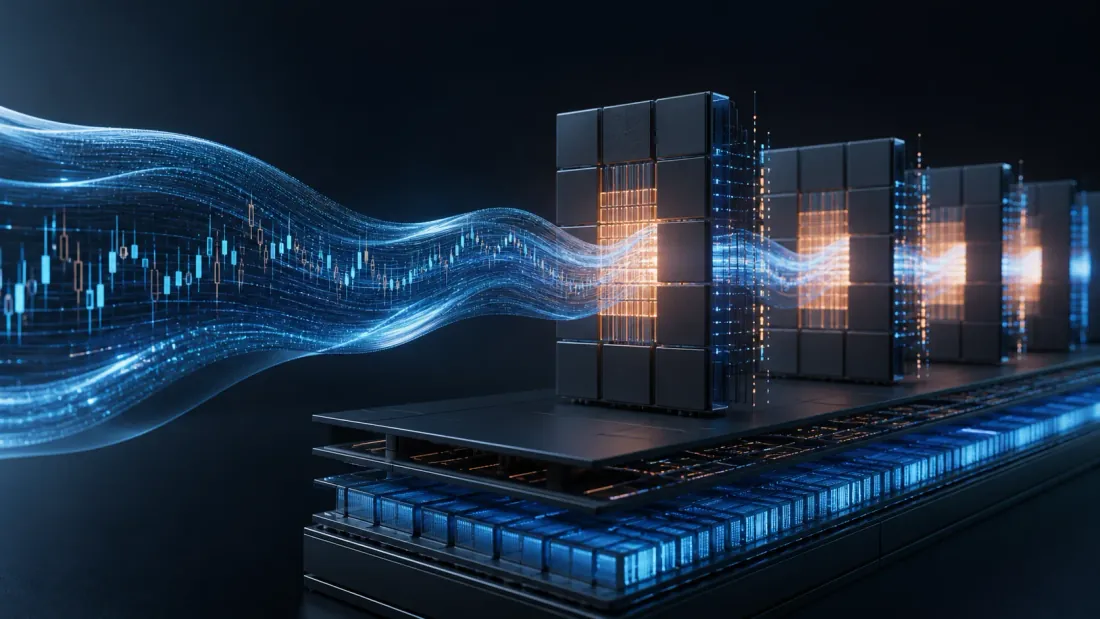
Aqui está a pergunta que este artigo existe para responder: se um transformador pudesse atender a um dia de negociação inteiro com resolução de um segundo em vez de uma janela de dez minutos, ele faria uma previsão melhor?
Até recentemente você nem conseguia perguntar. Necessidades de atenção padrão memória, portanto, um dia de 23.400 passos com 12 cabeças em float16 requer cerca de 12,9 GB apenas para a matriz de pontuação - mais do que os parâmetros do modelo e mais do que a maioria dos cartões oferece. A questão foi encerrada por aritmética antes que alguém pudesse testá-la.
Flash Attention (Dao et al., 2022) abre-o. Não aproximando a atenção - ele calcula exatamente o mesmo resultado - mas reestruturando a computação para ser consciente de IO, minimizando o tráfego entre os níveis de memória da GPU. Esse é o conteúdo genuinamente interessante aqui, e a maior parte deste artigo é dedicada a como ele funciona: lado a lado, a recorrência do softmax online, o Limite de IO e recomputação de passagem para trás.
Mas o mecanismo é o facilitador, não a reivindicação. "Um contexto mais longo é melhor" é uma afirmação empírica sobre os mercados e a posição deste blog - de Temporal Fusion Transformers, que descobriu que os transformadores vanilla em modelos recorrentes de overfit e short-lookback de séries financeiras permanecem competitivos em alta frequência – corta no sentido inverso. Portanto, o artigo termina na medição, não no mecanismo.
Por que a atenção está ligada à memória
Atenção computa — a própria primitiva, em um contexto de negociação, é abordada em Temporal Fusion Transformers for Multi-Horizon Portfolio Forecasting. Todo o problema é uma linha disso: a matriz de pontuação intermediária é , ele é gravado na memória, lido novamente para o softmax, gravado novamente e lido novamente para o matmul final - e deve ser mantido para retropropagação.
A intensidade aritmética da atenção é , então cerca de 64 FLOP/byte em — bem à esquerda do cume da A100. Ela fica no teto de largura de banda inclinado, não no teto de computação plano: a GPU passa mais tempo se movendo ao redor do que multiplicar qualquer coisa. A estrutura da linha do telhado usada - ponto de cumeeira, teto inclinado versus teto plano e por que o mesmo raciocínio decide se vale a pena comprar uma GPU - é construída com números medidos em Quando a GPU compensa.
A hierarquia de memória que o algoritmo explora
| Nível de memória | Tamanho | Largura de banda | Latência |
|---|---|---|---|
| HBM (memória de alta largura de banda) | 40-80 GB | 2,0 TB/s | ~400ns |
| SRAM (memória compartilhada no chip) | 20 MB | 19 TB/s | ~4 ns |
A SRAM tem aproximadamente 10x a largura de banda e 100x menos latência, com um milésimo da capacidade. Tudo o que o Flash Attention faz decorre dessa negociação: abrir mão de capacidade, comprar largura de banda e latência. O mesmo movimento de "reestruturar o algoritmo em vez de comprar hardware", medido em um backtest de CPU, é a escada de velocidade de backtest.
O algoritmo de atenção do Flash
Flash Attention processa a atenção em blocos dimensionados para caber na SRAM e nunca materializa a atenção completa matriz no HBM.
Partição em blocos de linha e em blocos de colunas, com escolhido de forma que uma peça e seus acumuladores caibam no chip. Para cada bloco de consulta, itere sobre todos os blocos de valores-chave:
For each query block Q_i:
    Initialize: O_i = 0, m_i = -inf, l_i = 0    # output, running max, running sum
    For each KV block (K_j, V_j):
        1. Load Q_i, K_j, V_j from HBM to SRAM
        2. Compute S_ij = Q_i @ K_j^T / sqrt(d)  # in SRAM
        3. Compute local max: m_ij = rowmax(S_ij)
        4. Compute P_ij = exp(S_ij - m_ij)        # in SRAM
        5. Compute local sum: l_ij = rowsum(P_ij)
        6. Update running statistics:
           m_new = max(m_i, m_ij)
           l_new = l_i * exp(m_i - m_new) + l_ij * exp(m_ij - m_new)
           O_i = O_i * (l_i * exp(m_i - m_new) / l_new)
                + P_ij @ V_j * (exp(m_ij - m_new) / l_new)
           m_i = m_new, l_i = l_new
    Write O_i to HBM
A recorrência do softmax online
O truque que torna possível o agrupamento é o softmax online. Um softmax ingênuo precisa de duas passagens na linha: uma para encontrar o máximo (para estabilidade numérica), outra para exponenciar e normalizar. Duas passagens em uma linha que você se recusa a armazenar são uma contradição - então o Flash Attention continua executando estatísticas e redimensionando conforme avança.
Depois dos blocos :
e o acumulador de saída é corrigido pelo mesmo fator:
Cada vez que um novo bloco aumenta o máximo de execução, a saída acumulada anteriormente é redimensionada retroativamente por – como se o novo máximo fosse conhecido desde o início. O resultado é algebricamente idêntico ao softmax de duas passagens. Na aritmética exata isto não é uma aproximação; é uma reassociação. (Em precisão finita, é um caminho de arredondamento diferente, o que importa - veja a verificação de exatidão abaixo.)
Complexidade de E/S
Esta é a declaração formal da vitória. Flash Atenção executa
Acessos HBM, onde é o tamanho da SRAM, contra para a implementação padrão. Observe que aparece no denominador: quanto maior o scratchpad no chip, menos viagens de ida e volta, e é por isso que o algoritmo é declarado em termos de hierarquia de memória e não de contagem de FLOP. Para típico e KB, a proporção favorece a atenção do Flash em cerca de 5 a 10 vezes menos acessos.
Passo para trás: recalcular em vez de armazenar
A retropropagação através da atenção normalmente precisa do matriz que o passe para frente simplesmente se recusou a manter. Flash Atenção recalcula os blocos de durante a passagem para trás, armazenando apenas a saída e as estatísticas softmax - ambos , não . Ele troca uma quantidade modesta de aritmética redundante pelo termo de memória que era o problema inteiro. Esta é a mesma barganha que o checkpoint de gradiente, aplicado na granularidade do bloco dentro de um único operador.
FA2: paralelismo
Flash Attention 2 (Dao, 2023) manteve o algoritmo e corrigiu o agendamento:
- Menos FLOPs não matmul. FA1 gastou tempo real em reescalonamento, localização máxima e exponenciação - operações que são executadas em núcleos CUDA, não em núcleos tensores. FA2 adia o reescalonamento até o final do loop interno.
- Paralelismo ao longo do comprimento da sequência. FA1 paraleliza apenas lotes e cabeçotes. FA2 também paraleliza blocos de consulta. Isso é importante especificamente para o caso de negociação, onde muitas vezes você tem uma sequência muito longa por ativo e um tamanho de lote de 1 a 4 – exatamente o regime em que o paralelismo de lote e cabeça deixa a GPU sem energia.
- Particionamento de trabalho de warp. Cada warp usa um subconjunto diferente de blocos de consulta em vez de dividir um cálculo de pontuação e reduzir entre warps, removendo uma redução de warp cruzada.
Resultado relatado: ~70% do pico teórico de FLOPs em A100 versus ~35% para FA1.
FA3: Mecânica da tremonha
Flash Attention 3 (Dao, Shah, 2024) é específico da arquitetura do H100:
- Especialização em warp assíncrona. O Tensor Memory Accelerator (TMA) de Hopper move HBM → SRAM de forma assíncrona. FA3 divide warps em produtores emitindo cargas TMA para o próximo bloco KV e consumidores computando no atual, de forma que a movimentação de dados se esconda atrás da aritmética.
- matmul e softmax intercalados. para um bloco é executado em núcleos tensores, enquanto o softmax para o bloco anterior é executado em núcleos CUDA - duas unidades de hardware diferentes, genuinamente simultâneas em vez de divididas no tempo.
- FP8 com processamento incoerente. H100 executa FP8 com taxa de transferência 2x FP16. A atenção ingênua do FP8 é prejudicada por valores discrepantes; FA3 gira vetores aleatoriamente antes da quantização em bloco para espalhar a magnitude atípica entre as coordenadas, relatado com erro numérico 2,6x menor do que o ingênuo FP8.
| Versão | GPU | Utilização | Aceleração vs Padrão |
|---|---|---|---|
| FA1 | A100 | ~35% | 2-4x |
| FA2 | A100 | ~70% | 5-7x |
| FA3 (FP16) | H100 | ~75% | 3-5x contra FA2 |
| FA3 (8º PQ) | H100 | ~75% | 1.6x contra FA3 FP16 |
O mascaramento causal é onde a negociação obtém um desconto
O mascaramento causal é obrigatório para séries temporais — o modelo não deve atender ao futuro — e sob o ladrilho não é um custo adicional, mas sim uma economia. Qualquer bloco cujas chaves estejam inteiramente no futuro em relação às suas consultas é ignorado imediatamente, nunca carregado e nunca computado, reduzindo aproximadamente metade do trabalho. No PyTorch isso é is_causal=True; nada mais é necessário.
A integração é de oito linhas
Quase nenhum código que você precisa é sobre Flash Attention. Troque o caminho explícito da matriz de pontuação pelo kernel fundido:
scores = torch.matmul(q, k.transpose(-2, -1)) / math.sqrt(d_head)
scores = scores.masked_fill(causal_mask, float("-inf"))
out = torch.matmul(torch.softmax(scores, dim=-1), v)

out = torch.nn.functional.scaled_dot_product_attention(
    q, k, v,
    dropout_p=self.dropout if self.training else 0.0,
    is_causal=True,
)
Essa é toda a mudança. q, k, v são moldados (batch, heads, seq, head_dim); a máscara causal desapareceu porque o kernel a constrói. Para um modelo de negociação PyTorch anotado completo para inserir isso - projeção de entrada, blocos e um cabeçote para cima/plano/para baixo de 3 classes - use DeepLOB e para obter um pipeline de treinamento completo, consulte Transformadores de fusão temporal. Construir uma quarta cópia desse andaime aqui não ensinaria nada.
Requisitos: capacidade de computação >= 8,0 (A100, H100, RTX 3090+), entradas de meia precisão, PyTorch >= 2,0. Verifique o atalho realmente utilizado torch.backends.cuda.sdp_kernel diagnóstico e torch.cuda.max_memory_allocated() - O SDPA retorna silenciosamente ao kernel matemático se alguma pré-condição falhar, e um substituto silencioso se parece exatamente com um modelo funcional que é meramente lento.
A medição: o contexto mais longo compensa?
Tudo acima diz que um contexto de 32K ou 128K agora é acessível. Não diz nada sobre se é útil. O experimento honesto:
Treine a mesma arquitetura em com SDPA-Flash na série BTC usada em outras partes desta série, mantendo parâmetros, otimizador e alvo fixos de forma que o comprimento da sequência seja a única variável. Relate duas coisas:
- Custo. Relógio de parede medido por época e
torch.cuda.max_memory_allocated()em cada . - Benefício. Desempenho preditivo fora da amostra versus , em uma divisão passo a passo.
Um rascunho anterior deste artigo trazia uma tabela de números de memória por comprimento de sequência derivados analiticamente do fórmula de ativação. Essas linhas foram removidas: elas nunca foram medidas e discordavam da aritmética do orçamento de memória do próprio artigo. Um número derivado apresentado em uma tabela de resultados é um resultado fabricado e este blog não os envia.
A propriedade interessante deste experimento é que ele pode ser publicado em qualquer direção. Se o desempenho fora da amostra aumentar monotonicamente com , isso justifica todo o programa de longo contexto. Se estagnar em alguns milhares de passos, ou se degradar, essa é uma peça mais forte - uma companheira do negativo honesto - e isso significaria que a parede da memória nunca foi a restrição vinculativa para a negociação de transformadores.
Mais contexto significa mais capacidade e, portanto, mais superfície de overfitting
Há uma razão específica para esperar um resultado estável ou negativo. Transformadores de Fusão Temporal já documenta que os transformadores vanilla se aplicam ingenuamente ao sobreajuste das séries financeiras — eles não possuem vieses indutivos temporais e os modelos recorrentes de retrospectiva curta permanecem competitivos em alta frequência. Estender o contexto de 512 para 32.768 passos não adiciona informações proporcionais ao comprimento; a defasagem marginal de 32.000 de uma série de preços quase eficiente tem muito pouco peso. O que ele adiciona de forma confiável é o valor dos parâmetros para ajustar.
Então a varredura deve ser tratado como realmente é: uma pesquisa de seleção de modelo, com o mesmo mecanismo que este blog aplica a todas as outras pesquisas. Três comprimentos de sequência vezes o que mais variar é uma contagem de teste, e o vencedor deve limpar uma Relação de Sharpe Deflacionada calculada contra essa contagem de teste e um portão PBO, e não apenas vencer seus vizinhos. Caso contrário, "vitórias de contexto longas" são indistinguíveis de escolher a melhor de três execuções barulhentas.
Uma verificação de exatidão, porque "exato" dá muito trabalho
A Atenção Flash é exata em aritmética exata. A recomendação anexada a ele – executar em FP16 ou bf16, e no H100 considerar FP8 – não é. Essas são afirmações separadas e a segunda domina na prática: reassociar uma soma e cair para metade da precisão são ambas perturbações, e o artigo que introduziu a garantia de ordenação não deveria então acenar com a mão a de precisão.
O blog já tem o instrumento certo. A armadilha de precisão da GPU estabelece o padrão: a baixa precisão não avisa, ela retorna lixo plausível e você prova a correção com um oráculo de paridade em uma quantidade discreta downstream – contagens de comércio – e não por curvas oculares. Aplicado aqui:
- Calcular atenção com SDPA-Flash em bf16 e com implementação de referência fp64 em entradas idênticas; relatar erro relativo máximo no tensor de saída.
- Leve-o até a decisão: para um modelo que emite um rótulo para cima/plano/para baixo, informe quantos rótulos mudam entre os dois caminhos, como uma fração do total de decisões.
Um desacordo pequeno, limitado e explicável é a assinatura de um caminho rápido correto. Um valor ilimitado significa que a recomendação do 8.º PQ nunca foi segura para este modelo. Nenhum dos números é conhecido até que seja executado.
Quando alcançá-lo
Comprimido na decisão, que tem o mesmo formato do Guia de decisão da GPU:
- Acima de ~2K passos de tempo em uma GPU CUDA: sim, incondicionalmente. É uma mudança de uma linha que produz saída exata, e a vitória cresce com . Não há cenário em que você queira que a materialização caminho em vez disso.
- Abaixo de aproximadamente 512 passos de tempo, na CPU ou com arquiteturas sem atenção (CNNs, SSMs como Mamba): irrelevante. À esquerda do cume, a sobrecarga fixa é o custo total e a atenção nunca foi seu gargalo.
- Os limites acima são folclore, não medição — eles vêm da literatura geral, e o crossover em seu próprio modelo e cartão é um benchmark de dez linhas. Execute-o em vez de confiar nos números redondos.
Conclusão
Flash Attention é um resultado limpo e genuinamente importante: respeitando a hierarquia de memória e reassociando o softmax, ele calcula a atenção exata com memória em vez de , e o O limite de IO explica exatamente o porquê. Adotá-lo em um transformador de negociação é uma mudança de uma linha, sem custo de precisão na aritmética exata e com um grande ganho de memória.
O que ele não faz é responder à pergunta no topo. Ele converte “um contexto de dia inteiro é impossível” em “um contexto de dia inteiro é barato”, o que representa uma mudança no custo do experimento, não no seu resultado. A queda do muro da memória é um convite à medição, e a medição é o que transforma isso de um resumo em papel em uma descoberta.
Referências
- Dao, T., Fu, DY, Ermon, S., Rudra, A., Re, C. "FlashAttention: Atenção exata rápida e com eficiência de memória com consciência de IO." NeurIPS (2022). arXiv:2205.14135
- Dao, T. "FlashAttention-2: Atenção mais rápida com melhor paralelismo e particionamento de trabalho." ICLR (2024). arXiv:2307.08691
- Dao, T., Shah, J. "FlashAttention-3: Atenção rápida e precisa com assincronia e baixa precisão." NeurIPS (2024). arXiv:2407.08608
- Vaswani, A., et al. "Atenção é tudo que você precisa." NeurIPS (2017).
- Milakov, M., Gimelshein, N. "Cálculo do normalizador online para softmax." arXiv:1805.02867 (2018).
Authors
Trading-systems engineer
Trading-systems engineer building bots since 2017: cross-exchange arbitrage (connected up to 30 venues), cointegration-based pairs arbitrage across spot and futures, scalping, news and sentiment-driven strategies, trend algorithms, and portfolio management and balancing algorithms. Also builds sub-millisecond order execution, big-data warehouses, backtesting engines, AI agents, and trading interfaces (incl. open-source profitmaker.cc). Stack: JS/TS, Python, Rust/Zig/Go, DevOps, backend, frontend, architecture.
Read More

Trade Classification When You Have No Side Flag: Tick, Quote, Lee-Ready, BVC

Tempo Irregular em Modelos de Tick: Codificações de Tempo Contínuo vs. Incorporações Posicionais Simples