Multi-Task Learning for Simultaneous Price, Volume, and Volatility Prediction
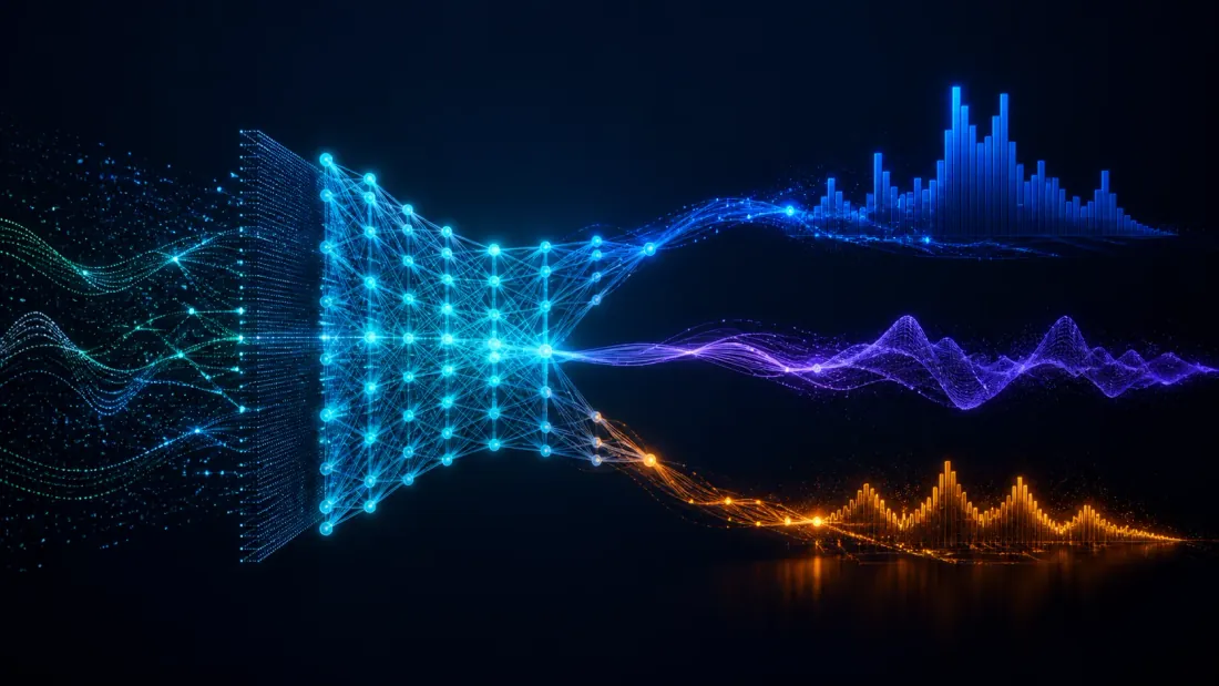
L'apprentissage multitâche (MTL) est généralement vendu avec une assertion : partagez un encodeur entre des cibles corrélées et la tâche principale s'améliore. Dans le trading, les objectifs corrélés sont évidents – les rendements, le volume et la volatilité réalisée découlent tous du même flux d’ordres – et cette affirmation n’est presque jamais testée. La question intéressante n’est pas de savoir si les tâches sont liées. Il s'agit de savoir si les dégradés partagés concordent et que se passe-t-il sur les plis là où ils ne le sont pas.
Cet article met deux éléments au centre que la plupart des articles de MTL traitent comme des notes de bas de page :
- L'équilibrage des pertes est une expérience, pas un détail. Les poids fixes, la pondération d'incertitude de Kendall et GradNorm sont trois modèles différents. Exécutez les trois sur les mêmes plis et signalez les poids appris ainsi que la métrique de la tâche principale pour chacun.
- Le transfert négatif est mesurable avant de voir la métrique. La similarité cosinusoïdale entre les gradients de tâches sur l'encodeur partagé vous indique, pendant la formation, si les tâches auxiliaires tirent la représentation quelque part où la tâche principale veut aller. Signez les cosinus, puis vérifiez si le signe prédit le résultat sur ce pli.
Tout le reste en cours – le processus de volatilité, la boucle de formation, les contrôles de fuite, le protocole de validation – est déjà couvert ailleurs sur ce blog et est lié plutôt que redérivé.
Configuration

Fonctionnalités d'entrée données (OHLCV, indicateurs techniques, flux de commandes), trois cibles :
- Tâche 1 (primaire) : retour de la période suivante
- Tâche 2 (auxiliaire) : volume du journal de la période suivante
- Tâche 3 (auxiliaire) : volatilité réalisée pour la période suivante
Un modèle multitâche produit les trois simultanément, , et le risque multitâche est une somme pondérée des risques par tâche :
L'intégralité de l'article porte sur et sur ce que les dégradés par tâche se font les uns aux autres.
Pourquoi une formation conjointe pourrait aider, en un paragraphe. Les tâches auxiliaires contraignent la représentation partagée à expliquer plus d'un phénomène de marché, qui est à la fois un contrôle de capacité et un biais inductif ; et comme le volume et la volatilité sont directement observés alors que le « retour attendu » ne l'est pas, les têtes auxiliaires fournissent un signal de gradient plus propre que la tête primaire. Les arguments en faveur d'un modèle émettant de nombreux résultats sont longuement argumentés - avec la machine d'interprétabilité attachée - dans [transformateurs de fusion temporels pour la prévision multi-horizon] (/en/blog/post/temporal-fusion-transformer-trading), qui présente le même argument d'encodeur partagé à plusieurs têtes pour les quantiles multi-horizons.
L'architecture, brièvement
Partage de paramètres dur : un encodeur partagé se nourrit chefs de tâches spécifiques , donc . Il s'agit de la version mesurée ici, car c'est la version où le dégradé est en conflit. est bien défini.
Partage de paramètres logiciel donne à chaque tâche son propre encodeur avec une pénalité de couplage - plus de paramètres, plus de flexibilité et pas de vecteur de paramètres partagés unique pour mesurer les conflits. Les réseaux de point de croix se situent entre les deux, mélangeant des fonctionnalités par tâche via une matrice apprise. à chaque niveau. Les deux valent la peine d’être essayés si le partage dur montre un conflit, et les deux sortent du champ d’application de la mesure ci-dessous.
L'expérience qui compte : trois systèmes d'équilibrage des pertes

La perte naïve est sensible à l’échelle. Si la perte de retour existe et perte de volume autour , le volume possède le dégradé et la tête de retour meurt de faim. Trois réponses :
Poids fixes. Ensemble après avoir standardisé chaque cible. La ligne de base honnête – s’il gagne, les programmes adaptatifs sont cérémonieux.
Pondération d'incertitude (Kendall et al., 2018). Apprenez une échelle de bruit homoscédastique par tâche :
Les tâches à forte incertitude sont automatiquement sous-pondérées ; le le terme bloque le trivial solution. Notez ceci est un dispositif de pondération de perte de temps d'entraînement, pas un intervalle prédictif — pour l'incertitude avec laquelle vous pouvez réellement dimensionner une position, voir prédiction conforme.
GradNorm (Chen et al., 2018). Équilibrez les magnitudes du gradient plutôt que les échelles de perte. Chaque étape : calculer et la moyenne , calculez le taux d'entraînement relatif , et mettre à jour . Toutes les tâches s'entraînent ensuite à des rythmes comparables, quelle que soit l'ampleur des pertes.
Le code spécifique à MTL correspond aux têtes, au retour de liste et à l'agrégation des pertes. La pile Linear/BatchNorm/ReLU/Dropout, le passe-partout Adam/cosinus/clip et la boucle d'époque sont le modèle standard présenté dans DeepLOB et sont omis ici.
import torch
import torch.nn as nn


class MultiTaskTradingModel(nn.Module):
    """Hard parameter sharing: one encoder, K heads."""

    def __init__(self, encoder: nn.Module, repr_dim: int, n_tasks: int = 3):
        super().__init__()
        self.shared_encoder = encoder          # any MLP/CNN/GRU trunk
        self.task_heads = nn.ModuleList(
            nn.Linear(repr_dim, 1) for _ in range(n_tasks)
        )

    def forward(self, x):
        h = self.shared_encoder(x)
        return [head(h).squeeze(-1) for head in self.task_heads]

    def shared_repr(self, x):
        return self.shared_encoder(x)


class UncertaintyWeightedLoss(nn.Module):
    """Kendall et al. (2018) homoscedastic weighting."""

    def __init__(self, n_tasks: int = 3):
        super().__init__()
        self.log_vars = nn.Parameter(torch.zeros(n_tasks))  # log(sigma^2)

    def forward(self, losses: list) -> torch.Tensor:
        return sum(
            torch.exp(-self.log_vars[i]) * loss + self.log_vars[i]
            for i, loss in enumerate(losses)
        )

    def get_weights(self) -> list:
        with torch.no_grad():
            return [torch.exp(-lv).item() for lv in self.log_vars]
UncertaintyWeightedLoss a des paramètres, il doit donc aller dans l'optimiseur à côté du modèle : optim.Adam(list(model.parameters()) + list(uw.parameters()), ...). Oublier cela est la manière la plus courante d'« exécuter une pondération d'incertitude » et d'exécuter silencieusement des poids fixes à la place.
Ce qu'il faut signaler
Pour chaque schéma, sur chaque pli : les poids finaux des tâches apprises, la métrique de la tâche principale et - parce qu'un schéma de pondération est un choix de modèle - combien de schémas ont été comparés avant d'en choisir un.
| Schéma | Métrique de tâche principale vs tâche unique | |||
|---|---|---|---|---|
| Fixé () | 1h00 | 1h00 | 1h00 | — |
| Pondération d'incertitude | — | — | — | — |
| Norme de diplôme | — | — | — | — |
Trois schémas fois plusieurs plis, c'est déjà une petite recherche de modèle. Toute amélioration signalée ici doit survivre à la correction des tests multiples décrite dans Sharpe dégonflé et tests multiples avant de signifier quoi que ce soit.
Transfert négatif : signez les dégradés

C'est la partie qui mérite d'être conservée. Le transfert négatif se produit lorsque les tâches auxiliaires aggravent la tâche principale et qu'il a un diagnostic direct : l'angle entre les gradients des tâches dans l'espace des paramètres partagés.
Mesuré uniquement sur l'encodeur partagé — les têtes sont spécifiques à une tâche par construction et sont toujours « d'accord » de manière triviale.
import torch.nn.functional as F


def shared_grad(model, x, y, task_idx, criterion=nn.MSELoss()):
    """Gradient of task `task_idx` w.r.t. the shared encoder, flattened."""
    model.zero_grad(set_to_none=True)
    loss = criterion(model(x)[task_idx], y)
    loss.backward()
    return torch.cat([
        p.grad.detach().flatten()
        for p in model.shared_encoder.parameters()
        if p.grad is not None
    ])


def task_conflict(model, x, y_by_task, task_names):
    """Pairwise cosine similarity between per-task shared-encoder gradients."""
    grads = {
        name: shared_grad(model, x, y_by_task[name], i)
        for i, name in enumerate(task_names)
    }
    return {
        (a, b): F.cosine_similarity(
            grads[a].unsqueeze(0), grads[b].unsqueeze(0)
        ).item()
        for i, a in enumerate(task_names)
        for b in task_names[i + 1:]
    }
Appelez cela sur un lot tenu à une cadence fixe pendant l'entraînement, pas une seule fois à la fin. Une paire peut commencer à s'aligner et diverger à mesure que l'encodeur se spécialise ; un seul numéro de fin de formation cache cela.
La découverte à rechercher – et à publier de toute façon :
| Paire | cos sim, formation précoce | cos sim, entraînement tardif | MTL a aidé à la tâche principale ? |
|---|---|---|---|
| retour ↔ volume | — | — | — |
| rendement ↔ volatilité | — | — | — |
| volume ↔ volatilité | — | — | — |
Si les gradients de volume et de volatilité s'accordent alors qu'ils sont tous deux en conflit avec le gradient de retour, la conclusion correcte est que les deux tâches auxiliaires forment un bloc cohérent auquel la tâche de retour n'appartient pas - et la solution est un regroupement de tâches, pas plus de capacité. Lorsque le conflit est réel, les remèdes standards sont PCGrad (Yu et al., 2020), qui projette chaque gradient conflictuel sur le plan normal de l'autre ; CAGrad (Liu et al., 2021), qui recherche une direction de descente qui ne nuit à aucune tâche ; ou abandonner complètement la tâche auxiliaire.
Notez ce qui est délibérément absent : un tracé t-SNE de la représentation partagée colorée par valeur cible. C'est décoratif - les nombres cosinus ci-dessus disent tout ce que l'intégration ferait geste, et ils le disent sous forme de nombres.
Protocole de validation

La mesure ci-dessus ne vaut rien avec un protocole bâclé, et MTL aggrave les pièges habituels car il y a trois cibles à fuir au lieu d'une.
Données réelles, pas un simulateur. Les cibles doivent provenir de données OHLCV/commerce réelles. Un jouet GARCH codé en dur génère une volatilité qui est corrélée aux rendements par construction, ce qui est précisément la chose testée : l'expérience mesurerait son propre générateur. Si vous souhaitez un processus de volatilité ajusté, Prévision de la volatilité GARCH pour la crypto s'adapte à GARCH(1,1) par maximum de vraisemblance sur le BTC/ETH réel et valide les résidus standardisés, et GARCH asymétrique et l'effet de levier explique pourquoi un simulateur gaussien à réponse symétrique déforme la volatilité de la crypto. en premier lieu. Les données synthétiques ne sont défendables que lorsqu’elles fournissent une vérité terrain contrôlée – une corrélation de tâches connue et définie par l’auteur que vous essayez de récupérer – ce qui est une expérience différente de celle ici.
Les scalers s'adaptent uniquement au train. Installez le scaler de fonctionnalités et les trois scalers cibles à l'intérieur de chaque pli d'entraînement et appliquez-les à la validation ; un mondial fit_transform avant de diviser les moments de test de fuite en entraînement. Cet échec exact est catalogué dans [la taxonomie des biais d'anticipation] (/en/blog/post/look-ahead-bias-taxonomy).
Pliages progressifs purgés et sous embargo. Une répartition chronologique 80/20 ne peut pas distinguer une amélioration MTL d'un effet de repliement - c'est tout l'argument de walk-forward enhancement, qui montre trois divisions produisant trois conclusions. Réutiliser la fenêtre extensible purged_walk_forward générateur de spread modeling with machine learning : il réduit un écart de horizon des lignes des deux côtés de chaque frontière, ce qui est important ici car les fenêtres de volatilité réalisée qui se chevauchent traversent la frontière même lorsque la cible de retour ne le fait pas.
Une ligne de base classique. Un filet MTL qui bat trois filets à tâche unique n'a rien prouvé si un modèle d'augmentation du gradient ou de crête par cible bat les quatre. Ajustez un modèle par cible avec LightGBM ou ridge sur les mêmes plis et les mêmes caractéristiques, et signalez-le dans le même tableau.
| Modèle | Métrique de la tâche principale | Remarques |
|---|---|---|
| Ridge, par cible | — | Ligne de base classique |
| LightGBM, par cible | — | Ligne de base classique |
| MLP à tâche unique, par cible | — | Trois filets séparés |
| MTL, meilleur plan de perte | — | Un filet, trois têtes |
Qu'est-ce qui ferait que MTL en vaut la peine ici

Conditions dans lesquelles MTL devrait gagner, énoncées sous forme d’hypothèses à vérifier par rapport aux plis ci-dessus plutôt que sous forme de liste de contrôle :
- Les étiquettes auxiliaires sont plus propres que l'étiquette principale. Le volume est directement observé ; Le "retour attendu" ne l'est pas. Si la tête de retour génère principalement du bruit, le signal de gradient provenant des têtes auxiliaires est la seule partie bien posée de l'objectif.
- Les données d'entraînement sont limitées par rapport à la capacité de l'encodeur, donc la contrainte auxiliaire effectue un véritable travail de régularisation plutôt que de simplement rivaliser pour les paramètres.
- La latence d'inférence est importante et une passe avant en bat trois.
Et les arguments contre, également vérifiables : si la valeur mesurée cos_sim(return, ·) les valeurs sont constamment négatives, l'encodeur partagé est éloigné de la tâche principale et les têtes auxiliaires sont une taxe, pas un régularisateur.
Conclusion

Les rendements, le volume et la volatilité proviennent de la même microstructure, donc une représentation partagée est un a priori raisonnable – mais un a priori n’est pas un résultat. Les deux choses que cette configuration peut réellement établir sont le schéma d'équilibrage des pertes que les données préfèrent (avec les poids appris rapportés, pas seulement le gagnant nommé) et si les gradients de tâches sur l'encodeur partagé concordent, mesurés au cours de l'entraînement plutôt que supposés du fait que les cibles sont corrélées.
Si les plis purgés montrent que le réseau MTL ne parvient pas à battre un modèle d'amélioration du gradient par cible, c'est la conclusion et elle est publiée en tant que telle - le modèle est [le négatif honnête] (/en/blog/post/honest-negative-no-robust-edge). Un résultat négatif sur un transfert négatif reste un résultat sur un transfert négatif.
Authors
Trading-systems engineer
Trading-systems engineer building bots since 2017: cross-exchange arbitrage (connected up to 30 venues), cointegration-based pairs arbitrage across spot and futures, scalping, news and sentiment-driven strategies, trend algorithms, and portfolio management and balancing algorithms. Also builds sub-millisecond order execution, big-data warehouses, backtesting engines, AI agents, and trading interfaces (incl. open-source profitmaker.cc). Stack: JS/TS, Python, Rust/Zig/Go, DevOps, backend, frontend, architecture.
Read More

Temps irrégulier dans les modèles de ticks : codages en temps continu par rapport aux intégrations positionnelles simples
Bid-Ask Spread Modeling and Prediction with Machine Learning