Koopman Operators and DMD: Do Market Modes Survive Out-of-Sample?

Dynamic Mode Decomposition sizga spectrum beradi: bir nechta complex eigenvalue, har birida o'sish rate'i va frequency'si, har biri asset cross-section ustidagi spatial mode'ga biriktirilgan. Bu structure'ga o'xshaydi. Asosiy savol — bu haqiqatan ham structuremi yoki linear operator noise'ning bitta window'ini sidqidildan yodlab olganmi.
Bu savolning tekshiriladigan ikki qismi bor va maqola shu ikki qism atrofida qurilgan:
- Mode persistence. DMD'ni window'ida va window'ida fit qiling. Dominant mode'lar bir xil subspace'ni qamrab oladimi yoki har bir refit'da qayta aralashadimi? Agar aralashsa, DMD in-sample decomposition'dan boshqa narsa emas — buni ochiq aytish yana bir tutorial'dan foydaliroq.
- Spectral radius leading indicator sifatida. Eng katta eigenvalue modulus'i fit qilingan dynamics qanchalik explosive ekanini jamlaydigan bitta scalar'dir. U realised volatility'ni oldindan yetaklaydimi, undan kechikadimi yoki shunchaki uni qayta aytadimi? Har ikkala javobni ham publish qilish mumkin; faqat birinchisi trade qilinadigan natija.
Bozorlar non-stationary nonlinear system'lar ekani bu yerda isbotlanmaydi, faraz qilinadi — blog buni allaqachon algotrading'dagi attractor'lar maqolasidagi phase-space geometry va HMM bilan regime detection dagi o'lchangan regime-specific BTC statistic'lari bilan ko'rsatgan. Quyidagi torroq savol — non-stationarity fit qilingan Koopman operatorga nima qilishi va buni qanday o'lchash.
1. Asosiy g'oya: nonlinear dynamics'ni linear qilish
State space dagi discrete-time dynamical system'ni ko'rib chiqing:
bu yerda ehtimol nonlinear map. Bozorlar uchun — vaqt qadamidagi asset return'lari, volatility'lari yoki order-book imbalance'laridan iborat vector.
Koopman operator state ning o'zida emas, scalar-valued observable function ustida ishlaydi:
Asosiy xususiyat: linear, hatto linear bo'lmasa ham. Buning narxi — dimensionality: infinite-dimensional function space'da ishlaydi. Yaxshi finite-dimensional approximation nonlinear dynamics ifodaliligini linear algebra boshqaruvchanligi bilan beradi: prediction matrix exponentiation'ga aylanadi va har bir mode network weight'lari ichiga ko'milmay, tekshiriladigan bo'ladi.
2. Koopman operator'ining spectral decomposition'i
Agar eigenvalue'lar va eigenfunction'lar ga ega bo'lsa, bo'ladi va shu eigenfunction'lar span'idagi har qanday observable quyidagicha decomposes:
bu yerda — Koopman mode'lari, har bir eigenfunction to'liq observable vector'ga qanday hissa qo'shishini tasvirlaydigan vector-valued coefficient'lar.
Har bir eigenvalue'i o'sish yoki decay rate'ini () va oscillation frequency'sini () kodlaydi:
| Komponent | Eigenvalue xususiyati | Moliyaviy talqin |
|---|---|---|
| Trend | , | Sekin drift, momentum |
| Cycle'lar | , | Oscillation'lar, seasonality |
| Transient'lar | So'nuvchi shock'lar, qisqa muddatli harakatlar | |
| Unstable mode'lar | O'suvchi, explosive dynamics |
Bu jadval va'dadir. 4-bo'limda va'da data bilan tekshiriladi.
3. Dynamic Mode Decomposition (DMD)
DMD data'dan 'ni approximate qilish uchun asosiy algorithm'dir. Matrix'lar ko'rinishida joylashtirilgan snapshot'lar berilganda:
DMD best-fit linear operator'ini sharti bilan izlaydi:
- SVD'ni hisoblang:
- Projection qiling:
- Eigendecomposition qiling:
- To'liq space mode'larini tiklang:
ustunlari DMD mode'lari, diagonali esa DMD eigenvalue'laridir.
import numpy as np
from numpy.linalg import svd, eig, lstsq

def dmd(X: np.ndarray, rank: int | None = None) -> tuple:
    """
    Dynamic Mode Decomposition.

    Parameters
    ----------
    X : np.ndarray, shape (n_features, n_snapshots)
        Data matrix where each column is a state snapshot.
    rank : int or None
        Truncation rank for the SVD. None = no truncation.

    Returns
    -------
    eigenvalues : np.ndarray, shape (r,)
        DMD eigenvalues (approximating Koopman eigenvalues).
    modes : np.ndarray, shape (n_features, r)
        DMD modes (columns), L2-normalised.
    amplitudes : np.ndarray, shape (r,)
        Mode amplitudes fitted to the FINAL snapshot, so that a one-step
        forecast is simply modes @ (eigenvalues * amplitudes).
    """
    X0 = X[:, :-1]
    X1 = X[:, 1:]

    U, S, Vh = svd(X0, full_matrices=False)

    if rank is not None:
        U = U[:, :rank]
        S = S[:rank]
        Vh = Vh[:rank, :]

    S_inv = np.diag(1.0 / S)

    A_tilde = U.conj().T @ X1 @ Vh.conj().T @ S_inv
    eigenvalues, W = eig(A_tilde)

    modes = X1 @ Vh.conj().T @ S_inv @ W

    norms = np.linalg.norm(modes, axis=0)
    norms[norms == 0] = 1.0
    modes = modes / norms

    amplitudes = lstsq(modes, X[:, -1].astype(complex), rcond=None)[0]

    return eigenvalues, modes, amplitudes
Bu yerda ikkita ataylab qilingan tanlov bor. Mode'lar L2-normalised, chunki 4.2-bo'lim window'lar bo'yicha mode subspace'larini solishtiradi va normalizatsiya qilinmagan amplitude'lar comparison'ni bosib ketishi mumkin. Amplitude'lar birinchi emas, oxirgi snapshot'ga fit qilinadi, demak forecast hech qachon eigenvalue'ni katta darajaga ko'tarmaydi — naive DMD signal'larini dynamics'ga o'xshatib qo'yadigan numerical blow-up aslida floating-point overflow'dir.
4. O'lchov
Maqolaning textbook'da bo'lmagan qismi shu. Yuqoridagilarning barchasi fitting procedure; quyida fit nimanidir anglatadimi-yo'qmi aniqlash protocol'i beriladi.
Data. Loyihaning o'z exchange data'sidan foydalaning — izchil minute yoki tick grid'dagi BTC, ETH va likvid alt'larning cross-section'i, equity ETF'larning daily download'i emas. Blog crypto-first, microstructure argument'i esa ko'chirilmaydi. 'ni asset'lar qatorlarda, time ustunlarda bo'ladigan qilib, log return'lar asosida, har bir window ichida asset bo'yicha demean qilingan holda tuzing.
4.1 Eigenvalue spectrum'i
Representative window uchun quyidagilarni report qiling: eigenvalue'dan nechtasi unit circle tolerance'i ichida, har biri soatlarda qaysi oscillation period'ga mos keladi (period bar, o'girilgan holda) va top mode return variance'ning qancha qismini reconstruct qiladi.
def spectrum_report(eigenvalues: np.ndarray, bar_minutes: float,
                    tol: float = 0.05) -> list[dict]:
    """
    Turn a DMD spectrum into human-readable rows: modulus, period in hours,
    and whether the eigenvalue sits on the unit circle within `tol`.
    """
    rows = []
    for lam in eigenvalues:
        modulus = float(np.abs(lam))
        omega = float(np.angle(lam))
        period_hours = (2 * np.pi / abs(omega)) * bar_minutes / 60 if omega else np.inf
        rows.append({
            "modulus": modulus,
            "period_hours": period_hours,
            "on_unit_circle": abs(modulus - 1.0) < tol,
            "regime": "unstable" if modulus > 1 + tol
                      else "persistent" if abs(modulus - 1.0) <= tol
                      else "decaying",
        })
    return sorted(rows, key=lambda r: -r["modulus"])


def reconstruction_r2(X: np.ndarray, modes: np.ndarray,
                      eigenvalues: np.ndarray, amplitudes: np.ndarray) -> float:
    """Fraction of in-window return variance captured by the truncated modes."""
    n_steps = X.shape[1]
    powers = eigenvalues[:, None] ** np.arange(-(n_steps - 1), 1)
    X_hat = (modes @ (amplitudes[:, None] * powers)).real
    resid = np.var(X - X_hat)
    return 1.0 - resid / np.var(X)
Halol spectrum report'ining o'zi maqolaga arziydi. Agar hech narsa unit circle yaqinida bo'lmasa, trade qilinadigan persistent cycle'lar yo'q va equity literature'dagi "annual seasonality" hikoyasi 24/7 crypto'ga shunchaki ko'chmaydi.
4.2 Qo'shni window'lar bo'yicha mode stability
Hal qiluvchi test. DMD'ni window'ida, keyin window'ida fit qiling va dominant mode subspace'ining qancha qismi saqlanishini o'lchang. To'g'ri statistic mode vector'larining naive correlation'i emas — mode ordering va complex phase ixtiyoriy — balki ikki subspace orasidagi principal angle'lardir.
def subspace_stability(modes_a: np.ndarray, modes_b: np.ndarray,
                       k: int = 3) -> float:
    """
    Overlap between the leading-k DMD mode subspaces of two adjacent windows.

    Returns the mean cosine of the principal angles: 1.0 = identical subspace,
    0.0 = orthogonal. Immune to mode reordering and complex phase, both of
    which are arbitrary in a DMD fit.
    """
    Qa, _ = np.linalg.qr(modes_a[:, :k])
    Qb, _ = np.linalg.qr(modes_b[:, :k])
    sing = np.linalg.svd(Qa.conj().T @ Qb, compute_uv=False)
    return float(np.mean(np.clip(sing, 0.0, 1.0)))


def stability_curve(returns: np.ndarray, window: int, step: int,
                    rank: int, k: int = 3) -> np.ndarray:
    """Subspace overlap between every pair of adjacent windows."""
    fits = []
    for t_end in range(window, returns.shape[1], step):
        evals, modes, _ = dmd(returns[:, t_end - window:t_end], rank=rank)
        order = np.argsort(-np.abs(evals))
        fits.append(modes[:, order])
    return np.array([subspace_stability(fits[i], fits[i + 1], k=k)
                     for i in range(len(fits) - 1)])
Shu overlap distribution'ini va uni null bilan solishtirib report qiling: ayni return'larning phase-randomised surrogate'larida hisoblangan shu statistic. Yuqori, ammo surrogate null'dan yuqori bo'lmagan overlap mode'lar dynamics'ni emas, covariance structure'ni kuzatayotganini bildiradi.
4.3 Realised volatility'ga nisbatan rolling spectral radius
Tekshiriladigan da'vo: rolling window'larda qayta hisoblangan realised volatility bilan birga emas, undan oldin harakat qiladi. Scalar mexanik jihatdan yangi emas — blog ilgari geometric scalar'larni real vaqtda, xususan algorithmic trading uchun complex manifold'lar maqolasidagi Kobayashi curvature'ni kuzatgan — ammo Koopman eigenvalue modulus'i boshqa failure mode'ga ega boshqa quantity'dir va meros qilib olingan pitch emas, o'z lead-lag test'iga loyiq.
def rolling_spectral_radius(returns: np.ndarray, window: int = 1440,
                            step: int = 60, rank: int = 5) -> dict:
    """
    Rolling DMD spectrum for regime monitoring.

    returns : np.ndarray, shape (n_assets, n_timesteps)
    window  : rolling window length in bars
    step    : bars between refits
    """
    idx, radii, dom_freq = [], [], []

    for t_end in range(window, returns.shape[1], step):
        X_win = returns[:, t_end - window:t_end]
        try:
            evals, _, _ = dmd(X_win, rank=rank)
        except np.linalg.LinAlgError:
            continue

        idx.append(t_end)
        radii.append(float(np.max(np.abs(evals))))

        on_circle = np.abs(np.abs(evals) - 1.0) < 0.1
        if on_circle.any():
            sel = evals[on_circle]
            dom_freq.append(float(np.abs(np.angle(sel[np.argmax(np.abs(sel))])) / (2 * np.pi)))
        else:
            dom_freq.append(0.0)

    return {"index": np.array(idx),
            "spectral_radius": np.array(radii),
            "dominant_frequency": np.array(dom_freq)}


def lead_lag(signal: np.ndarray, target: np.ndarray, max_lag: int = 24) -> dict:
    """
    Cross-correlation of `signal` against `target` over +/- max_lag steps.
    A peak at negative lag means the signal LEADS the target.
    """
    s = (signal - signal.mean()) / (signal.std() + 1e-12)
    y = (target - target.mean()) / (target.std() + 1e-12)
    lags = np.arange(-max_lag, max_lag + 1)
    corrs = []
    for L in lags:
        if L < 0:
            corrs.append(float(np.corrcoef(s[:L], y[-L:])[0, 1]))
        elif L > 0:
            corrs.append(float(np.corrcoef(s[L:], y[:-L])[0, 1]))
        else:
            corrs.append(float(np.corrcoef(s, y)[0, 1]))
    corrs = np.array(corrs)
    return {"lags": lags, "corr": corrs, "peak_lag": int(lags[np.argmax(np.abs(corrs))])}
Align spectral_radius'ni ayni grid'da hisoblangan realised volatility bilan align qiling va peak_lag'ni o'qing. Lag 0 dagi peak qo'shimcha qadamlar bilan aytilgan volatility restatement ekanini bildiradi. Sample bo'ylab va rank'lar bo'ylab barqaror negative lag'dagi peak — maqoladagi trade qilinadigan da'voga ega yagona variant.
Ijobiy natijadan keyin nima bo'lishi haqida
Agar oldindan yetaklasa, keyingi obvious qadam cross-sectional construction bo'ladi: asset'larni DMD bashorat qilgan next-step return bo'yicha rank qiling, bashorat qilingan winner'larda long, loser'larda short bo'ling. Bu construction bu yerda yangi emas — u crypto'da statistical arbitrage va pairs trading hamda vector va matrix'lar bilan complex arbitragening 4-bo'limida yoritilgan factor-residual trade; haqiqiy Koopman-specific twist faqat eigenportfolio'lar static PCA loading'lari o'rniga time-varying eigenvalue'larni olib yurishidir.
Strategy section'i bu maqolada ataylab yo'q, chunki u bu yerda fees va slippage bilan backtest qilinmagan. Qilinganda, blogning o'z mezonidan o'tishi kerak: Deflated Sharpe Ratio va multiple testing dagi significance test'i va honest negativening doimiy counter-example'iga qarshi. DMD spectrum plot'i result emas.
One-step forecast'ning o'zi uchun to'g'ri implementation eigenvalue'ni window length darajasiga ko'tarish o'rniga oxirgi snapshot'dan bashorat qiladi:
def dmd_one_step(returns: np.ndarray, rank: int = 4) -> np.ndarray:
    """
    One-step-ahead prediction from the final snapshot of the window.

    Never raise eigenvalues to the window length: any |lambda| != 1 then
    overflows or underflows and the "signal" becomes numerical garbage.
    """
    evals, modes, amplitudes = dmd(returns, rank=rank)
    return (modes @ (evals * amplitudes)).real
5. Extended DMD (EDMD): nonlinear observable'lar
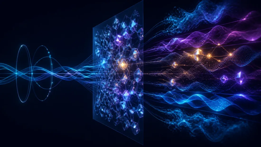
Standard DMD xom state vector ustida ishlaydi. EDMD avval data'ni nonlinear basis function'lar dictionary'si orqali lift qiladi.
dictionary'i scalar function'laridan iborat bo'lganda, lifted state'ni quyidagicha aniqlang:
EDMD 'ni sharti bilan izlaydi. Quyidagi code ishlatadigan convention'da — state'lar column sifatida, chapdan ta'sir qiladi:
| Dictionary turi | Function'lar | Nimani qamrab oladi |
|---|---|---|
| Polynomial | Nonlinear cross-asset interaction'lar | |
| Radial basis (RBF) | Mahalliy o'xshashlik, regime clustering'i | |
| Time-delay embedding | Xotira / autoregressive structure | |
| Fourier | Ma'lum periodicity'lar (intraday, weekly) | |
| Volatility feature'lari | Heteroskedasticity, vol clustering |
Dictionary domain knowledge kiradigan joy, time-delay row esa delay coordinate'lar haqida umuman qayg'urishning Koopman-specific sababidir: ular alohida ulab qo'yilgan technique emas, lifting map'ning yana bir block'idir. Embedding'ning o'zi — delay , embedding dimension tanlovi va uning ortidagi reconstruction theorem — algorithmic trading uchun complex manifold'larda allaqachon kiritilgan va code qilingan; u yerdagi delay vector'larni oling va qo'shimcha row sifatida to'g'ridan-to'g'ri build_financial_dictionary'ga uzating.
import numpy as np
from itertools import combinations_with_replacement

def build_financial_dictionary(X: np.ndarray, max_poly_degree: int = 2,
                               include_volatility: bool = True,
                               delay_steps: int = 0) -> np.ndarray:
    """
    Build a dictionary of nonlinear observables for EDMD.

    X : np.ndarray, shape (n_features, n_snapshots)
    Returns Z of shape (n_dict, n_snapshots - delay_steps).
    """
    n_features, n_snapshots = X.shape
    offset = max(delay_steps, 0)
    X_eff = X[:, offset:]
    n_eff = X_eff.shape[1]

    lifted = [X_eff]  # degree-1 terms (identity)

    if max_poly_degree >= 2:
        for deg in range(2, max_poly_degree + 1):
            for combo in combinations_with_replacement(range(n_features), deg):
                term = np.ones(n_eff)
                for idx in combo:
                    term *= X_eff[idx]
                lifted.append(term.reshape(1, -1))

    if include_volatility:
        lifted.append(np.abs(X_eff))   # absolute returns
        lifted.append(X_eff ** 2)      # squared returns

    for d in range(1, delay_steps + 1):
        lifted.append(X[:, offset - d : n_snapshots - d])

    return np.vstack(lifted)


def edmd(X: np.ndarray, dictionary_fn=None, reg: float = 1e-8,
         **dict_kwargs) -> tuple:
    """
    Extended Dynamic Mode Decomposition.

    Solves Z1 ~= K @ Z0 in the least-squares sense. Uses a least-squares
    solve rather than an explicit Gram inverse: `inv` on a near-singular
    dictionary Gram matrix is how EDMD spectra get silently corrupted.
    """
    if dictionary_fn is None:
        dictionary_fn = lambda x: build_financial_dictionary(x, **dict_kwargs)

    Z = dictionary_fn(X)
    Z0, Z1 = Z[:, :-1], Z[:, 1:]

    p = Z0.shape[0]
    G = Z0 @ Z0.T + reg * np.eye(p)   # regularised Gram matrix
    A = Z1 @ Z0.T

    K = np.linalg.solve(G, A.T).T

    eigenvalues, eigenvectors = np.linalg.eig(K)
    return K, eigenvalues, eigenvectors
6. Deep Koopman network'lari
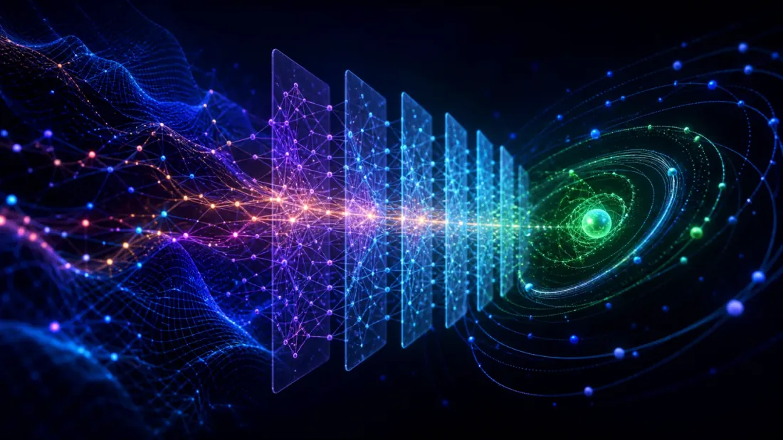
EDMD dictionary'si qo'lda yaratiladi, bu Koopman-invariant subspace noma'lum bo'lganda haqiqiy cheklovdir. Deep Koopman network'lari lifting va operator'ni birgalikda o'rganadi.
Architecture autoencoder'dir — encoder, latent code, decoder, reconstruction loss, barchasi algotrading'da anomaly detectionda kiritilgan — unga bu bo'limning butun mohiyati bo'lgan bitta qo'shimcha qo'shiladi: latent dynamics'ni bitta o'rganilgan matrix'i orqali majburlaydigan linearity loss.
x_k  -->  [Encoder φ]  -->  z_k  -->  [Linear K]  -->  z_{k+1}  -->  [Decoder ψ]  -->  x̂_{k+1}
                              |                            |
                              +--- Linearity loss: ‖z_{k+1} - K z_k‖ ---+
term'isiz latent space'i matrix multiply'dan keyin keladigan oddiy autoencoder bo'ladi. U bilan network evolution'i linear bo'lmagan har qanday latent representation uchun jarimaga tortiladi — o'rganilgan 'ni Koopman approximation'iga va uning eigenvalue'larini 4-bo'limdagi DMD spectrum'iga taqqoslanadigan qiladigan narsa shu.
import torch
import torch.nn as nn

class DeepKoopman(nn.Module):
    """Deep Koopman autoencoder: learned lifting + linear latent dynamics."""

    def __init__(self, input_dim: int, latent_dim: int, hidden_dim: int = 128):
        super().__init__()

        self.encoder = nn.Sequential(
            nn.Linear(input_dim, hidden_dim), nn.ReLU(),
            nn.Linear(hidden_dim, hidden_dim), nn.ReLU(),
            nn.Linear(hidden_dim, latent_dim),
        )
        self.decoder = nn.Sequential(
            nn.Linear(latent_dim, hidden_dim), nn.ReLU(),
            nn.Linear(hidden_dim, hidden_dim), nn.ReLU(),
            nn.Linear(hidden_dim, input_dim),
        )
        self.K = nn.Linear(latent_dim, latent_dim, bias=False)

    def encode(self, x: torch.Tensor) -> torch.Tensor:
        return self.encoder(x)

    def decode(self, z: torch.Tensor) -> torch.Tensor:
        return self.decoder(z)

    def forward(self, x_k: torch.Tensor) -> dict:
        z_k = self.encode(x_k)
        z_k1_pred = self.K(z_k)
        return {
            "z_k": z_k,
            "z_k1_pred": z_k1_pred,
            "x_k1_pred": self.decode(z_k1_pred),
            "x_k_recon": self.decode(z_k),
        }

    def multi_step_predict(self, x_0: torch.Tensor, n_steps: int) -> torch.Tensor:
        """Roll out by repeated application of the linear operator."""
        z = self.encode(x_0)
        preds = []
        for _ in range(n_steps):
            z = self.K(z)
            preds.append(self.decode(z))
        return torch.stack(preds, dim=1)

    def latent_spectrum(self) -> np.ndarray:
        """Eigenvalues of the learned K — directly comparable to DMD's."""
        return np.linalg.eigvals(self.K.weight.detach().cpu().numpy())


def koopman_loss(model: DeepKoopman, x_k: torch.Tensor, x_k1: torch.Tensor,
                 alpha: float = 1.0, beta: float = 0.5) -> torch.Tensor:
    out = model(x_k)
    z_k1_true = model.encode(x_k1)

    prediction = nn.functional.mse_loss(out["x_k1_pred"], x_k1)
    linearity = nn.functional.mse_loss(out["z_k1_pred"], z_k1_true)
    reconstruction = nn.functional.mse_loss(out["x_k_recon"], x_k)

    return prediction + alpha * linearity + beta * reconstruction
latent_spectrum buni sequence model'ga o'tish o'rniga o'qitishga arziydigan qiladi: o'rganilgan operator hali ham matrix, shuning uchun 4.2-bo'limdagi stability test va 4.3-bo'limdagi lead-lag test deep model'ga o'zgarishsiz qo'llanadi.
7. Amaliy mulohazalar va xatolar
Rank tanlovi. Truncation rank'i bias-variance dial'idir — juda past bo'lsa dynamics o'tkazib yuboriladi, juda yuqori bo'lsa noise'ga fit qilinadi. Singular-value elbow'ga ko'z bilan qaramang; blog vector va matrix'lar bilan complex arbitrageda Random Matrix Theory'dagi Marchenko-Pastur bound bilan "noise'ga fit qilishdan oldin nechta component kerak" savoliga allaqachon to'g'ri javob bergan. Singular value'lari window shape uchun Marchenko-Pastur edge'dan oshadigan component'larni saqlang va natijaviy 'ni publish qiladigan har bir spectrum yonida aniq ko'rsating.
Window length. Koopman theory fixed 'ni faraz qiladi, bozorlar esa bitta operator bermaydi. Rolling refit'lar majburiy, 4.2-bo'limdagi stability curve tanlangan window estimate qilish uchun yetarlicha uzun va bitta regime ichida qolish uchun yetarlicha qisqami-yo'qmi tekshiradigan ayni diagnostic'dir.
Noise sensitivity. Financial data signal-to-noise ratio'si past, standard DMD esa dagi noise sabab biased bo'ladi. Mode'lar unstable degan xulosaga kelishdan oldin sinashga arziydigan remedy'lar:
- Total DMD (TDMD) — total least squares orqali va ning ikkalasini ham noisy deb qaraydi.
- Optimized DMD — eigenvalue-mode decomposition'ni residual Frobenius norm'iga nisbatan to'g'ridan-to'g'ri optimallashtiradi.
- Kernel EDMD — dictionary qurmasdan high-dimensional feature space'da implicit ishlaydi.
Agar TDMD ostida mode stability sezilarli oshsa, instability measurement noise bo'lgan. Oshmasa, sabab bozor bo'lgan.
8. DMD qayerda joylashadi

| Method | Linearity | Interpretable | Multi-step forecast |
|---|---|---|---|
| DMD | State space'da linear | Ha (mode'lar + eigenvalue'lar) | Stable (matrix power) |
| EDMD | Lifted space'da linear | Ha, dictionary berilganda | Stable (matrix power) |
| Deep Koopman | O'rganilgan space'da linear | O'rtacha (latent K'ni tekshirish) | Stable (matrix power) |
Volatility-specific forecasting uchun taqqoslash nuqtasi GARCH family'sidir — crypto uchun GARCH volatility forecastingga qarang. To'liq nonlinear sequence model'lar va ular olib keladigan interpretability hamda error-accumulation trade-off'lari uchun trading'dagi Temporal Fusion Transformerga qarang.
DMD egallagan niche tor, ammo haqiqiy: autoregressive rollout o'rniga bitta matrix power orqali hosil qilingan multi-step forecast'lar, har bir mode'ni tekshirish mumkin. Bu niche alpha'ga egami — 4-bo'limning savoli, bu jadvalniki emas.
Xulosa

Koopman theory bozor dynamics'iga qarashning haqiqatan ham nafis usuli, aynan shu nafislik sabab eng qattiq mavjud testga muhtoj. Asosiy xulosalar:
- DMD'ni fit qiling va fit'ni darhol test qiling. Adjacent window'lar orasidagi subspace overlap'ni phase-randomised null bilan solishtirib o'lchash bir tushdan keyin structure topdingizmi yoki window'ni yodladingizmi, aytib beradi.
- Rolling spectral radius kuzatishga arziydigan yagona scalar, uning qiymati esa butunlay lead-lag result'iga bog'liq. Lag 0 da u volatility proxy, negative lag'da regime warning.
- Amplitude'larni oxirgi snapshot'ga anchor qiling va eigenvalue'larni hech qachon window length darajasiga ko'tarmang. Amaliyotdagi DMD "signal"larining katta qismi floating-point artifact'lardir.
- Rank'ni elbow'ga ko'z bilan qarab emas, Marchenko-Pastur orqali tanlang va har bir spectrum bilan rank'ni publish qiling.
- Spectrum plot'i result emas. Shu ustiga qurilgan har qanday strategy hisobga kirishidan oldin fees, slippage va deflated Sharpe test'idan o'tishi kerak.
Bu variantlardan tashqari implementation'lar uchun PyDMD library DMD variant'larini to'liq qamrab oladi, Mallen et al.'ning reference code'i esa deep Koopman qismini qamrab oladi.
Bozorlar tartibsiz, non-stationary va qisman kuzatiladigan bo'lib qoladi. Koopman theory shu tartibsizlikdan structure ajratib olish uchun principled lens beradi — keyingi hafta ham structure saqlanganini tekshirsangiz.
Manbalar va qo'shimcha o'qish:
- B. O. Koopman, "Hamiltonian Systems and Transformation in Hilbert Space," Proceedings of the National Academy of Sciences, 1931.
- J. H. Tu et al., "On Dynamic Mode Decomposition: Theory and Applications," Journal of Computational Dynamics, 2014.
- M. O. Williams, I. G. Kevrekidis, C. W. Rowley, "A Data-Driven Approximation of the Koopman Operator: Extending Dynamic Mode Decomposition," Journal of Nonlinear Science, 2015.
- B. Lusch, J. N. Kutz, S. L. Brunton, "Deep Learning for Universal Linear Embeddings of Nonlinear Dynamics," Nature Communications, 2018.
- J. Mann and J. N. Kutz, "Dynamic Mode Decomposition for Financial Trading Strategies," Quantitative Finance, 2016.
- A. Mallen et al., "Koopman Neural Forecaster for Time Series with Temporal Distribution Shifts," ICML, 2023.
- E. Gonzalez and M. Generelo, "Analysis of chaotic economic models through Koopman operators, EDMD, Takens' theorem and Machine Learning," Data Science in Finance and Economics, 2022.
Authors
Trading-systems engineer
Trading-systems engineer building bots since 2017: cross-exchange arbitrage (connected up to 30 venues), cointegration-based pairs arbitrage across spot and futures, scalping, news and sentiment-driven strategies, trend algorithms, and portfolio management and balancing algorithms. Also builds sub-millisecond order execution, big-data warehouses, backtesting engines, AI agents, and trading interfaces (incl. open-source profitmaker.cc). Stack: JS/TS, Python, Rust/Zig/Go, DevOps, backend, frontend, architecture.
Read More

XGBoost for Return Direction: Class Imbalance and Decision Thresholds

Irregular Time in Tick Models: Continuous-Time Encodings vs. Plain Positional Embeddings