व्यवस्थित ट्रेडिंग पाइपलाइनों के लिए ऑटोएमएल
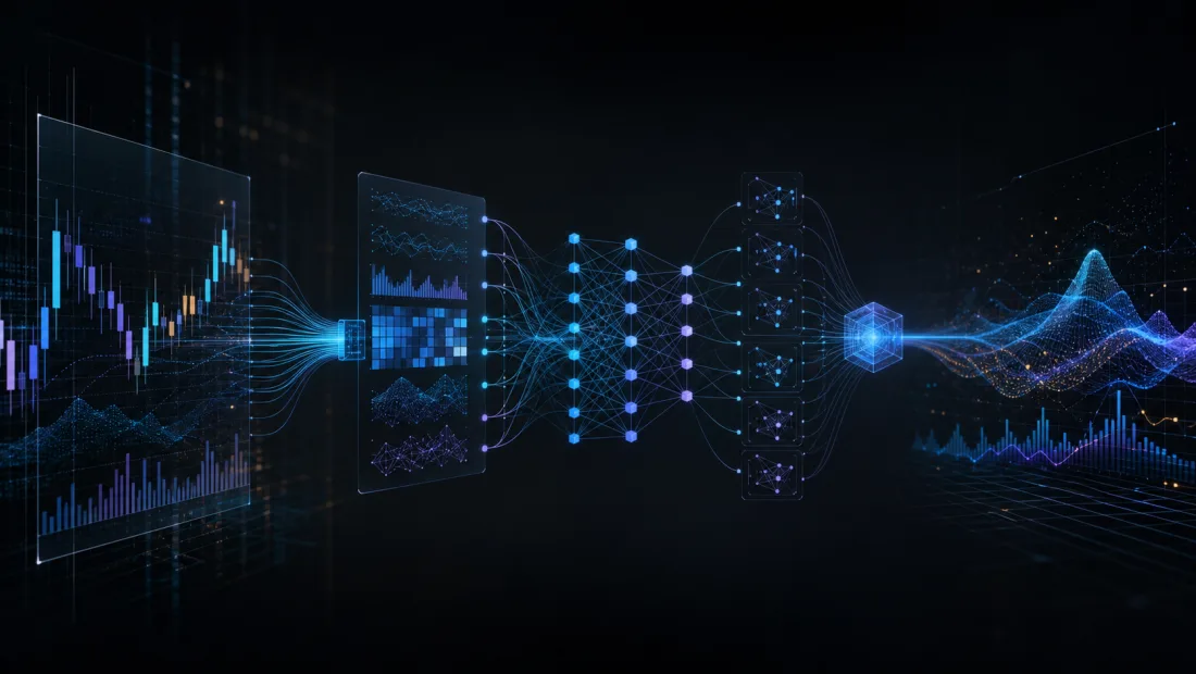
इस ब्लॉग ने खोज कैसे करें पर एक लंबी चर्चा की है: किस नमूने का उपयोग करना है और कब (ZXQKEEP0QXZ), आपके द्वारा की गई खोज की कीमत कैसे तय करें (ZXQKEEP1QXZ), चयन प्रक्रिया को कैसे स्कोर करें (ZXQKEEP2QXZ), और वह संपूर्ण उपकरण वास्तव में कहां पहुंचता है (ZXQKEEP3QXZ)।
जो चीज़ इसमें कभी शामिल नहीं हुई वह वही है जो आप ओवर खोजते हैं। वे सभी लेख दिए गए फीचर सेट और रणनीति परिवार को लेते हैं और इसके अंदर मापदंडों को अनुकूलित करते हैं। ऑटोएमएल ऊपर की परत पर हमला करता है - यह स्वयं उम्मीदवारों के निर्माण को स्वचालित करता है। इसके तीन भाग इस ब्लॉग पर कहीं और नहीं दिखते:
- स्वचालित फ़ीचर निष्कर्षण - tsfresh एक मूल्य श्रृंखला को ~794 सांख्यिकीय रूप से चित्रित सुविधाओं में बदलना, और फ़ीचरटूल्स डीप फ़ीचर सिंथेसिस के माध्यम से संबंधित बाज़ार तालिकाओं में सुविधाओं की रचना करना।
- बजट-जागरूक ऑटोएमएल - एफएलएएमएल का लागत-मितव्ययी अनुकूलन, जो लागत की परवाह किए बिना गणना बजट के भीतर सबसे अच्छा मॉडल ढूंढता है।
- फॉर्मूलाइक अल्फा फैक्ट्री - वर्ल्डक्वांट के 101 फॉर्मूलाइक अल्फाज एक कंपोजेबल ऑपरेटर व्याकरण के रूप में एक मशीन की गणना कर सकते हैं।
बाकी सब कुछ - वस्तुनिष्ठ कार्य, सत्यापन योजना, बहु-परीक्षण सुधार - पहले से ही यहां कहीं और मापा जाता है, इसलिए यह लेख फिर से सिखाने के बजाय लिंक करता है। यह सामान्य से अधिक मायने रखता है, क्योंकि ऑटोएमएल ट्रायल गिनती को विस्फोटित कर देता है, और ट्रायल गिनती बिल्कुल वही है जो बाकी चाप के बारे में है।
! ZXQKEEP0QXZ
ऑटोएमएल क्या स्वचालित करता है
AutoML कोई एकल एल्गोरिदम नहीं है. यह तकनीकों का एक परिवार है जो पाइपलाइन के विभिन्न चरणों को स्वचालित करता है:
| स्टेज | मैनुअल दृष्टिकोण | ऑटोएमएल दृष्टिकोण |
|---|---|---|
| फ़ीचर इंजीनियरिंग | डोमेन विशेषज्ञ शिल्प संकेतक | स्वचालित निष्कर्षण (टीएसफ्रेश, फीचरटूल्स) |
| फ़ीचर चयन | सहसंबंध विश्लेषण, अंतर्ज्ञान | सांख्यिकीय परिकल्पना परीक्षण, SHAP |
| मॉडल चयन | 2-3 मॉडल आज़माएं | दर्जनों शिक्षार्थियों को खोजें |
| हाइपरपैरामीटर ट्यूनिंग | ग्रिड खोज, मैनुअल ट्विकिंग | बायेसियन / लागत-मितव्ययी खोज (ऑप्टुना, FLAML) |
| वास्तुकला डिजाइन | फिक्स्ड न्यूरल नेटवर्क टोपोलॉजी | तंत्रिका वास्तुकला खोज (एनएएस) |
| पहनावा निर्माण | मैनुअल स्टैकिंग | स्वचालित पहनावा चयन |
आधार यह है कि व्यवस्थित व्यापार में उम्मीदवार का स्थान बहुत बड़ा है - एक एकल ओएचएलसीवी श्रृंखला सैकड़ों तकनीकी विशेषताएं उत्पन्न करती है, और कई संपत्तियां, ऑर्डर बुक डेटा और वैकल्पिक स्रोत इसे संयोजित बनाते हैं। आधार भी ख़तरा है: प्रत्येक उम्मीदवार एक परीक्षण है, और परीक्षण ही झूठी खोजों का निर्माण करते हैं।
उद्देश्य पर एक ऑटोएमएल-विशिष्ट बिंदु: खोज जिस मीट्रिक को अधिकतम करती है वह वित्तीय होनी चाहिए, क्योंकि खोज वही अनुकूलित करेगी जो आपने लिखा था और आपका कोई मतलब नहीं था। आप जो स्केलर चुनते हैं वह चुपचाप आपकी रणनीति का चयन करता है - ZXQKEEP1QXZ देखें, जहां एक अनुभवहीन प्रति-ट्रेड शार्प 600 बीजों में से 56% में उप-5%-एक्सपोजर लॉटरी का ताज जीतता है और 21 का एक इन-सैंपल शार्प पोस्ट करता है जो सैंपल में से 0.13 पर गिर जाता है। प्रारंभ से ही वित्तीय मीट्रिक को ऑटोएमएल स्कोरर से जोड़ें; ZXQKEEP0QXZ को अनुकूलित न करें और आशा करें कि यह स्थानांतरित हो जाएगा।
स्वचालित फ़ीचर इंजीनियरिंग
फ़ीचर इंजीनियरिंग वह जगह है जहाँ अधिकांश अल्फ़ा रहते हैं। कच्चा मूल्य डेटा सभी के लिए समान है। उस डेटा का पूर्वानुमानित संकेतों में परिवर्तन लाभदायक रणनीतियों को शोर से अलग करता है।
! ZXQKEEP0QXZ
tsfresh: एक मूल्य श्रृंखला से लेकर 800+ सुविधाओं तक
ZXQKEEP0QXZ (स्केलेबल हाइपोथिसिस टेस्ट पर आधारित टाइम सीरीज़ फ़ीचर एक्सट्रैक्शन) टाइम सीरीज़ फ़ीचर निष्कर्षण के उद्देश्य से बनाया गया है। यह 63 लक्षण वर्णन विधियों की गणना करता है जो डिफ़ॉल्ट रूप से ~794 सुविधाओं में विस्तारित होते हैं, जिनमें शामिल हैं:
- सांख्यिकीय क्षण (माध्य, विचरण, तिरछापन, कर्टोसिस)
- एकाधिक अंतराल पर स्वत:सहसंबंध
- फूरियर गुणांक और वर्णक्रमीय ऊर्जा
- जटिलता उपाय (अनुमानित एन्ट्रापी, नमूना एन्ट्रापी)
- अरेखीय विशेषताएं (फ्रेडरिक गुणांक, अधिकतम लैंग्विन निश्चित बिंदु)
- मात्राएँ और सीमा गणनाएँ बदलें
वित्तीय डेटा के लिए, इसका मतलब है कि एक एकल मूल्य श्रृंखला सैकड़ों उम्मीदवार सुविधाओं का उत्पादन करती है - कई कैप्चरिंग डायनामिक्स जो मैन्युअल फीचर इंजीनियरिंग में छूट जाएंगी। यह ZXQKEEP0QXZ और ZXQKEEP1QXZ में उपयोग किए गए हस्त-निर्मित, डोमेन-व्युत्पन्न फीचर सेट से एक भौतिक रूप से अलग दृष्टिकोण है: वहां एक मानव निर्णय लेता है कि ऑर्डर-बुक असंतुलन मायने रखता है; यहां एक पुस्तकालय हर चीज़ की गणना करता है और एक परिकल्पना परीक्षण को निर्णय लेने देता है। For financial data, this means a single price series produces hundreds of candidate features — many capturing dynamics that manual feature engineering would miss. This is a materially different approach from the hand-crafted, domain-derived feature sets used in spread modeling and DeepLOB : there a human decides that order-book imbalance matters; here a library enumerates everything and lets a hypothesis test decide.
import pandas as pd
import numpy as np
from tsfresh import extract_features, select_features
from tsfresh.utilities.dataframe_functions import impute

def prepare_rolling_windows(df: pd.DataFrame, window_size: int = 20) -> pd.DataFrame:
    """Convert OHLCV DataFrame into rolling windows for tsfresh."""
    records = []
    for i in range(window_size, len(df)):
        window = df.iloc[i - window_size:i].copy()
        window["id"] = i  # window identifier
        window["time"] = range(window_size)
        records.append(window[["id", "time", "close", "volume", "high", "low"]])
    return pd.concat(records, ignore_index=True)

df_ohlcv = pd.read_csv("btc_1h.csv", parse_dates=["timestamp"])
df_rolled = prepare_rolling_windows(df_ohlcv, window_size=24)

features = extract_features(
    df_rolled,
    column_id="id",
    column_sort="time",
    n_jobs=8,  # parallel extraction
    disable_progressbar=False,
)

impute(features)

y = df_ohlcv["close"].pct_change(4).shift(-4).iloc[24:].reset_index(drop=True)
y_binary = (y > 0).astype(int)

features_selected = select_features(features, y_binary, fdr_level=0.05)
print(f"Selected {features_selected.shape[1]} features from {features.shape[1]}")
ZXQKEEP0QXZ फ़ंक्शन संपूर्ण फीचर बैटरी में गलत खोज दर को नियंत्रित करने के लिए बेन्जामिनी-येकुटिएली प्रक्रिया लागू करता है - जो कि सही वृत्ति है, और वही वृत्ति ZXQKEEP1QXZ रणनीति खोजों पर लागू होती है। ध्यान दें कि यह क्या नहीं करता है: सुविधा-चयन चरण पर एफडीआर नियंत्रण इसके बाद आने वाले मॉडल खोज की परीक्षण लागत के बारे में कुछ नहीं कहता है। वे दो अलग-अलग गुण हैं और दोनों का भुगतान करना होगा।
फ़ीचरटूल्स: डीप फ़ीचर सिंथेसिस
जबकि tsfresh समय श्रृंखला लक्षण वर्णन पर ध्यान केंद्रित करता है, ZXQKEEP0QXZ रिलेशनल फीचर इंजीनियरिंग में उत्कृष्टता प्राप्त करता है - संबंधित तालिकाओं में आदिम संचालन की रचना करके सुविधाओं का निर्माण करता है।
ट्रेडिंग के लिए, यह तब शक्तिशाली होता है जब आपके पास मल्टी-टेबल डेटा हो: व्यापार इतिहास, ऑर्डर बुक स्नैपशॉट, फंडिंग दरें और ऑन-चेन मेट्रिक्स। फ़ीचरटूल्स डीप फ़ीचर सिंथेसिस (डीएफएस) लागू करता है, जो परिवर्तन और एकत्रीकरण प्राइमेटिव्स को ढेर करता है: For trading, this is powerful when you have multi-table data: trade history, order book snapshots, funding rates, and on-chain metrics. Featuretools applies Deep Feature Synthesis (DFS), which stacks transformation and aggregation primitives:
import featuretools as ft

es = ft.EntitySet(id="crypto_trading")

es = es.add_dataframe(
    dataframe_name="candles",
    dataframe=df_candles,
    index="candle_id",
    time_index="timestamp",
)

es = es.add_dataframe(
    dataframe_name="orderbook",
    dataframe=df_orderbook,
    index="snapshot_id",
    time_index="timestamp",
)

es = es.add_dataframe(
    dataframe_name="funding",
    dataframe=df_funding,
    index="funding_id",
    time_index="timestamp",
)

feature_matrix, feature_defs = ft.dfs(
    entityset=es,
    target_dataframe_name="candles",
    agg_primitives=["mean", "std", "max", "min", "skew", "trend"],
    trans_primitives=["percentile", "diff", "cum_mean"],
    max_depth=2,  # compose up to 2 primitives deep
    features_only=False,
)

print(f"Generated {len(feature_defs)} features via DFS")
ZXQKEEP0QXZ घोषणा लोड-असर वाली है: यह वह है जो फ़ीचरटूल्स को केवल कटऑफ पर मौजूद पंक्तियों का उपयोग करके एकत्रीकरण की गणना करने देती है। इसे गलत समझें और DFS खुशी-खुशी भविष्य में एक फीचर बनाएगा - ZXQKEEP1QXZ में सूचीबद्ध लीक का रिलेशनल-डेटा उदाहरण।
tsfresh (समय श्रृंखला लक्षण वर्णन) और फ़ीचरटूल्स (रिलेशनल सिंथेसिस) का संयोजन आपको एक फ़ीचर फ़ैक्टरी देता है जो बिना किसी मैन्युअल संकेतक कोडिंग के कच्चे बाज़ार डेटा से हजारों उम्मीदवार सिग्नल तैयार करता है।
बजट-अवेयर ऑटोएमएल: एफएलएएमएल
हम ऑप्टुना और ट्री-स्ट्रक्चर्ड पारज़ेन एस्टीमेटर्स को पृष्ठभूमि के रूप में मानते हैं - व्युत्पत्ति, नमूना तुलना और बेंचमार्क ZXQKEEP0QXZ में हैं। किस नमूने तक पहुंचना है, इस ब्लॉग का अपना माप संदर्भ है और यह लोककथाओं का उत्तर नहीं है: क्रॉसओवर मूल्यांकन लागत द्वारा शासित होता है, न कि एल्गोरिदम चतुराई से - जब एक बैकटेस्ट लगभग मुफ़्त होता है, तो स्क्रैम्बल सोबोल थ्रूपुट पर जीत जाता है (टीपीई के लिए ~154 के मुकाबले ~2,830 सीएफजी/एस), और केवल महंगे मूल्यांकन नमूना दक्षता भुगतान (ZXQKEEP1QXZ) करते हैं।
! ZXQKEEP0QXZ
वह फ़्रेमिंग ही FLAML को प्रतिस्पर्धी सैंपलर के बजाय एक अलग धुरी बनाती है। ऑप्टुना पूछता है अगला नमूना कहाँ लेना है; ZXQKEEP0QXZ (फ़ास्ट लाइटवेट ऑटोएमएल) पूछता है मैं आख़िर क्या नमूना ले सकता हूँ। यह एक समय के भीतर सर्वश्रेष्ठ मॉडल के लिए अनुकूलन करता है या सीएफओ (लागत-मितव्ययी अनुकूलन) का उपयोग करके बजट की गणना करता है, जो शुरुआती मूल्यांकन के लिए सस्ते कॉन्फ़िगरेशन को प्राथमिकता देता है और केवल तभी बढ़ता है जब अनुमानित सीमांत लाभ खर्च को उचित ठहराता है। That framing is what makes FLAML a different axis rather than a competing sampler. Optuna asks where to sample next; FLAML (Fast Lightweight AutoML) asks what can I afford to sample at all. It optimizes for the best model within a time or compute budget using CFO (Cost-Frugal Optimization), which prioritizes cheap-to-evaluate configurations early and escalates only when the estimated marginal gain justifies the spend.
from flaml import AutoML
from sklearn.metrics import make_scorer
import numpy as np

def sharpe_score(y_true, y_pred):
    """Custom scorer: Sharpe ratio of predicted signals."""
    signal = np.sign(y_pred - 0.5)
    returns = signal * y_true  # y_true contains forward returns
    if returns.std() == 0:
        return 0.0
    return np.sqrt(252) * returns.mean() / returns.std()

sharpe_scorer = make_scorer(sharpe_score, greater_is_better=True)

automl = AutoML()
automl_settings = {
    "time_budget": 300,          # 5 minutes
    "metric": sharpe_scorer,     # optimize the financial objective, not accuracy
    "task": "classification",
    "estimator_list": [
        "lgbm", "xgboost", "rf", "extra_tree", "catboost",
    ],
    "eval_method": "cv",
    "split_type": "time",        # time series split (no future leakage)
    "n_splits": 5,
    "log_file_name": "flaml_trading.log",
    "seed": 42,
}

automl.fit(
    X_train=X_train,
    y_train=y_train,
    **automl_settings,
)

print(f"Best model: {automl.best_estimator}")
print(f"Best config: {automl.best_config}")

from flaml.data import get_output_from_log
time_history, best_valid_loss_history, valid_loss_history, config_history, metric_history = \
    get_output_from_log(filename="flaml_trading.log", time_budget=300)
ट्रेडिंग के लिए FLAML का लाभ विभिन्न मॉडल प्रकारों में आवंटन की गणना करना है। यदि लाइटजीबीएम कॉन्फ़िगरेशन कैटबूस्ट की तुलना में 10 गुना तेजी से मूल्यांकन करता है, तो एफएलएएमएल जल्दी ही अधिक लाइटजीबीएम की खोज करता है और केवल तभी स्विच करता है जब यह अनुमान लगाता है कि सीमांत सुधार लागत को उचित ठहराता है। यह क्रॉसओवर लेख से सस्ते-शासन की अंतर्दृष्टि है, सामान्यीकृत: थ्रूपुट खोज बजट में प्रथम श्रेणी का शब्द है, न कि कार्यान्वयन विवरण।
प्रक्षेप पथ लॉग रखने लायक हिस्सा है। ZXQKEEP0QXZ आपको पूर्ण कॉन्फ़िगरेशन इतिहास देता है, जो आपकी परीक्षण गणना है - और परीक्षण गणना आपके द्वारा देय प्रत्येक अपस्फीति का इनपुट है।
ट्रेडिंग मॉडल के लिए तंत्रिका वास्तुकला खोज
न्यूरल आर्किटेक्चर सर्च किसी निश्चित की ट्यूनिंग के बजाय नेटवर्क टोपोलॉजी के डिज़ाइन को स्वचालित करता है। वित्तीय श्रृंखला के लिए वास्तुकला का विकल्प वास्तव में गैर-स्पष्ट है - गैर-स्थिरता, कम सिग्नल-टू-शोर, मिश्रित आवृत्तियों और मिनटों से महीनों तक फैली निर्भरताएं सभी अलग-अलग दिशाओं में खींचती हैं - लेकिन प्रेरणा पहले से ही कहीं और ठोस रूप से तर्क दी गई है: जब टीएफटी एलएसटीएम को हराता है तो ZXQKEEP0QXZ देखें, वेनिला ट्रांसफार्मर को हराता है, और सीएनएन + इंसेप्शन + एलएसटीएम ट्रेडऑफ़ पर ZXQKEEP1QXZ देखें, जो सावधानीपूर्वक हाथ से डिज़ाइन किया गया है। आर्किटेक्चर पहले ही हासिल कर चुके हैं। एनएएस का तर्क है कि इस विकल्प को स्वयं खोजा जाना चाहिए।
ZXQKEEP0QXZ पर शोध से पता चलता है कि RNN EXAMM (एवोल्यूशनरी एक्सप्लोरेशन ऑफ ऑगमेंटिंग मेमोरी मॉडल्स) के माध्यम से विकसित हुए हैं, जिन्होंने सरल लॉन्ग-शॉर्ट रणनीतियों का उपयोग करके भालू (2022) और बुल (2023) दोनों बाजारों में डीजेआई और एस एंड पी 500 से बेहतर प्रदर्शन किया है। इसे तीसरे पक्ष के दावे के रूप में मानें, न कि यहां पुनरुत्पादित परिणाम के रूप में - यह खोज में सबसे अच्छा आंकड़ा है, जिसमें कोई अपस्फीति रिपोर्ट नहीं की गई है।
NAS ट्रेडिंग के लिए स्थान खोजें
ट्रेडिंग मॉडल के लिए एक व्यावहारिक NAS खोज स्थान में शामिल हैं: A practical NAS search space for trading models includes:
Search Space:
  - Cell types: {LSTM, GRU, Temporal Conv, Transformer block, Linear}
  - Number of layers: [1, 8]
  - Hidden dimensions: {32, 64, 128, 256}
  - Attention heads (if Transformer): {2, 4, 8}
  - Dropout rate: [0.0, 0.5]
  - Skip connections: {True, False}
  - Normalization: {BatchNorm, LayerNorm, None}
  - Activation: {ReLU, GELU, SiLU, Mish}
  - Lookback window: {20, 60, 120, 252}
माइक्रोसॉफ्ट के एनएनआई (न्यूरल नेटवर्क इंटेलिजेंस) के साथ, आप इस स्थान को परिभाषित और खोज सकते हैं: With NNI (Neural Network Intelligence) from Microsoft, you can define and search this space:
import nni
from nni.nas.nn.pytorch import LayerChoice, InputChoice
import torch
import torch.nn as nn

class TradingNASModel(nn.Module):
    """NAS-searchable model for financial time series."""

    def __init__(self, input_dim: int, seq_len: int):
        super().__init__()
        self.input_proj = nn.Linear(input_dim, 128)

        self.temporal_block = LayerChoice([
            nn.LSTM(128, 128, num_layers=2, batch_first=True, dropout=0.1),
            nn.GRU(128, 128, num_layers=2, batch_first=True, dropout=0.1),
            nn.TransformerEncoder(
                nn.TransformerEncoderLayer(d_model=128, nhead=4, batch_first=True),
                num_layers=2,
            ),
        ], label="temporal_cell")

        self.head = LayerChoice([
            nn.Sequential(nn.Linear(128, 64), nn.ReLU(), nn.Linear(64, 1)),
            nn.Sequential(nn.Linear(128, 32), nn.GELU(), nn.Linear(32, 1)),
            nn.Linear(128, 1),
        ], label="prediction_head")

        self.skip = InputChoice(n_candidates=2, n_chosen=1, label="skip_conn")
        self.skip_proj = nn.Linear(input_dim, 128)

    def forward(self, x: torch.Tensor) -> torch.Tensor:
        h = self.input_proj(x)
        out = self.temporal_block(h)

        if isinstance(out, tuple):
            out = out[0]

        last = out[:, -1, :]

        skip_val = self.skip_proj(x[:, -1, :])
        last = self.skip([last, last + skip_val])

        return self.head(last).squeeze(-1)
खोज एल्गोरिदम (ENAS, DARTS, या इवोल्यूशनरी) एक वित्तीय उद्देश्य का उपयोग करके सत्यापन सेट पर उम्मीदवार आर्किटेक्चर का मूल्यांकन करता है, फिर उत्तरोत्तर उच्च-प्रदर्शन टोपोलॉजी की ओर बढ़ता है। इस लेख में बाकी सभी चीजों के मुकाबले लागत विषमता पर ध्यान दें: एनएएस मूल्यांकन-लागत अक्ष के सबसे महंगे छोर पर बैठता है, जो एक ऐसा शासन है जहां नमूना-कुशल नमूने और बहु-निष्ठा छंटाई वास्तव में खुद के लिए भुगतान करती है।
वर्ल्डक्वांट अल्फा फ़ैक्टरी दृष्टिकोण
अल्फा डिस्कवरी के लिए वर्ल्डक्वांट का दृष्टिकोण वित्त में ऑटोएमएल सिद्धांतों का सबसे औद्योगिक पैमाने पर कार्यान्वयन है। इगोर तुलचिंस्की द्वारा स्थापित, वर्ल्डक्वांट वह संचालित करता है जिसे वे "अल्फा फैक्ट्री" कहते हैं - लाखों पूर्वानुमानित संकेतों को उत्पन्न करने, परीक्षण करने और संयोजन करने की एक व्यवस्थित प्रक्रिया।
दर्शन: घातीय अल्फा पीढ़ी, और इसका सुधार
वर्ल्डक्वांट ने 2010 में दस लाख अल्फ़ाज़ तक पहुंचने का लक्ष्य रखा था, उस समय जब वे प्रति वर्ष केवल कई हज़ार अल्फ़ाज़ का उत्पादन करते थे। उन्होंने 2016 में उस लक्ष्य को हासिल किया। यह दर्शन सक्रिय प्रबंधन के मौलिक नियम पर आधारित है:
ZXQKEEP0QXZ
जहां ZXQKEEP0QXZ सूचना अनुपात है, ZXQKEEP1QXZ सूचना गुणांक है, और ZXQKEEP2QXZ चौड़ाई है - स्वतंत्र दांव की संख्या। प्रत्येक व्यक्ति ZXQKEEP3QXZ एक कमजोर भविष्यवक्ता है; दावा यह है कि कमजोर रूप से सहसंबद्ध पर्याप्त आईसी को मिलाकर छोटे आईसी को एक सार्थक जोखिम-समायोजित रिटर्न में बदल दिया जाता है।
सुधार जो इसे बनाता या तोड़ता है, और सूत्र का अनुभवहीन पाठ छिपाता है: चौड़ाई परीक्षण गणना नहीं है। ZXQKEEP1QXZ स्वतंत्र दांवों की गणना करता है, और उत्पन्न अल्फ़ाज़ स्वतंत्र नहीं होते हैं - वे समान मूल्य और वॉल्यूम फ़ील्ड पर समान ऑपरेटरों से बने होते हैं, इसलिए वे एक-दूसरे की सहसंबंध संरचना को प्राप्त करते हैं। इस ब्लॉग ने प्रभाव को सीधे ZXQKEEP0QXZ में मापा: प्रभावी चौड़ाई ZXQKEEP2QXZ है, और एक विशिष्ट क्रिप्टो सहसंबंध कारक ZXQKEEP3QXZ के साथ, दस सिग्नल लगभग 3.3 स्वतंत्र के लायक हैं। ZXQKEEP4QXZ शब्द आपके द्वारा जेनरेट किए गए अल्फ़ाज़ के आधार पर नहीं बढ़ता है; यह इस बात से बढ़ता है कि कितने असंबंधित जीवित बचे हैं। एक लाख सहसंबद्ध अल्फ़ाज़ आपको विज्ञापित फ़ॉर्मूले की तुलना में बहुत कम कीमत पर खरीदते हैं।
यही कारण है कि नीचे दिया गया चरण 3 - मौजूदा लाइब्रेरी के विरुद्ध सजावट - अल्फा फैक्ट्री में एक स्वच्छता कदम नहीं है। यह वह कदम है जो सबसे पहले चौड़ाई पैदा करता है।
101 सूत्रीय अल्फ़ाज़
काकुशाद्ज़े (वर्ल्डक्वांट रिसर्च से जुड़े) के पेपर ZXQKEEP0QXZ ने फॉर्मूलाइक अल्फा अभिव्यक्तियों का एक सेट प्रकाशित किया - मूल्य, मात्रा और मौलिक डेटा पर गणितीय अभिव्यक्तियाँ: The paper "101 Formulaic Alphas" by Kakushadze (associated with WorldQuant research) published a set of formulaic alpha expressions — mathematical expressions over price, volume and fundamental data:
Alpha#1:  (rank(Ts_ArgMax(SignedPower(((returns < 0) ? stddev(returns, 20)
          : close), 2.), 5)) - 0.5)

Alpha#7:  ((adv20 < volume) ? ((-1 * ts_rank(abs(delta(close, 7)), 60))
          * sign(delta(close, 7))) : (-1 * 1))

Alpha#42: (rank(vwap - close) / rank(vwap + close))
ऑटोएमएल के लिए जो बात इसे दिलचस्प बनाती है वह यह है कि यह एक व्याकरण है। अल्फ़ाज़ एक छोटे फ़ील्ड सेट (ZXQKEEP6QXZ, ZXQKEEP7QXZ, ZXQKEEP8QXZ) पर एक छोटे ऑपरेटर सेट (ZXQKEEP0QXZ, ZXQKEEP1QXZ, ZXQKEEP2QXZ, ZXQKEEP3QXZ, ZXQKEEP4QXZ, ZXQKEEP5QXZ) की रचनाएँ हैं। , ZXQKEEP9QXZ , ZXQKEEP10QXZ ). एक व्याकरण गणना योग्य है, जिसका अर्थ है कि खोज स्थान इस तरह से मशीन-जनरेट करने योग्य है कि "एक अच्छी सुविधा के बारे में सोचें" नहीं है। एक ऑटोएमएल प्रणाली यह कर सकती है:
- डेटा फ़ील्ड पर ऑपरेटरों की रचना करके उम्मीदवार अभिव्यक्तियाँ उत्पन्न करें
- प्रत्येक अभिव्यक्ति के आईसी, टर्नओवर और ड्रॉडाउन का मूल्यांकन करें
- उन अभिव्यक्तियों के लिए फ़िल्टर जो सांख्यिकीय परीक्षण में जीवित रहते हैं और मौजूदा लाइब्रेरी के साथ पर्याप्त रूप से असंबंधित हैं
- बचे हुए लोगों को एक पोर्टफोलियो में मिलाएं
ध्यान दें कि चरण 1 और 2 आसान हैं और चरण 3 वह है जहां मूल्य है - ऊपर चौड़ाई सुधार देखें।
एलएलएम-एन्हांस्ड अल्फा डिस्कवरी
वर्ल्डक्वांट ने बड़े भाषा मॉडल को अल्फा फैक्ट्री में एकीकृत करना शुरू कर दिया है। जैसा कि वित्तीय प्रेस में बताया गया है, फर्म यह पता लगा रही है कि एलएलएम कैसे "विभिन्न डोमेन में अल्फ़ाज़ को बदल और खोज सकते हैं" - उपन्यास अभिव्यक्तियाँ उत्पन्न करना, शोध पत्रों को परीक्षण योग्य परिकल्पनाओं में अनुवाद करना, और क्रॉस-डोमेन रिश्तों को सामने लाना जो एक शुद्ध गणनात्मक खोज से छूट जाएंगे। यह पाठ से सिग्नल निकालने से एक अलग तंत्र है, जिसे यह ब्लॉग ZXQKEEP0QXZ में शामिल करता है; यहां एलएलएम फॉर्मूला लिखता है, फीचर नहीं।
अपनी खुद की मिनी अल्फा फैक्ट्री का निर्माण
यहां ऑपरेटर व्याकरण पर एक संक्षिप्त लेकिन कार्यात्मक अल्फा फैक्ट्री है: Here is a compact but functional alpha factory over the operator grammar:
import itertools
from dataclasses import dataclass
from typing import Callable, List
import pandas as pd
import numpy as np
from scipy.stats import spearmanr

@dataclass
class Alpha:
    name: str
    expression: Callable[[pd.DataFrame], pd.Series]
    ic: float = 0.0
    turnover: float = 0.0
    sharpe: float = 0.0

def ts_rank(series: pd.Series, window: int) -> pd.Series:
    return series.rolling(window).apply(lambda x: pd.Series(x).rank().iloc[-1] / len(x))

def ts_delta(series: pd.Series, period: int) -> pd.Series:
    return series.diff(period)

def ts_std(series: pd.Series, window: int) -> pd.Series:
    return series.rolling(window).std()

def cs_rank(series: pd.Series) -> pd.Series:
    return series.rank(pct=True)

def ts_mean(series: pd.Series, window: int) -> pd.Series:
    return series.rolling(window).mean()

ALPHA_TEMPLATES = [
    ("momentum_{w}",
     lambda df, w: cs_rank(ts_delta(df["close"], w))),
    ("mean_reversion_{w}",
     lambda df, w: -cs_rank(df["close"] / ts_mean(df["close"], w) - 1)),
    ("vol_surprise_{w}",
     lambda df, w: cs_rank(df["volume"] / ts_mean(df["volume"], w))),
    ("price_vol_divergence_{w}",
     lambda df, w: cs_rank(ts_delta(df["close"], w)) * -cs_rank(ts_delta(df["volume"], w))),
    ("volatility_rank_{w}",
     lambda df, w: -cs_rank(ts_std(df["close"].pct_change(), w))),
    ("high_low_range_{w}",
     lambda df, w: cs_rank(ts_mean(df["high"] - df["low"], w) / df["close"])),
]

WINDOWS = [5, 10, 20, 60, 120]

def generate_alphas(df: pd.DataFrame, forward_returns: pd.Series) -> List[Alpha]:
    """Generate and evaluate all alpha candidates."""
    alphas = []

    for (name_tpl, expr_fn), window in itertools.product(ALPHA_TEMPLATES, WINDOWS):
        name = name_tpl.format(w=window)
        try:
            signal = expr_fn(df, window)
            signal = signal.replace([np.inf, -np.inf], np.nan)

            valid = signal.notna() & forward_returns.notna()
            if valid.sum() < 100:
                continue

            ic, _ = spearmanr(signal[valid], forward_returns[valid])
            turnover = signal.diff().abs().mean()

            ret = (signal * forward_returns).dropna()
            sharpe = np.sqrt(252) * ret.mean() / (ret.std() + 1e-9)

            alphas.append(Alpha(
                name=name,
                expression=lambda df, fn=expr_fn, w=window: fn(df, w),
                ic=ic,
                turnover=turnover,
                sharpe=sharpe,
            ))
        except Exception:
            continue

    alphas.sort(key=lambda a: abs(a.ic), reverse=True)
    return alphas
पांच विंडो पर छह टेम्पलेट एक 30-कॉन्फ़िगरेशन स्वीप है। यह जो रिपोर्ट तैयार करता है उसका योजनाबद्ध आकार होता है - फ़ील्ड वे हैं जो फ़ैक्टरी उत्सर्जित करती है, और कोई संख्या नहीं भरी जाती है क्योंकि यहां किसी को भी मापा नहीं गया है: Six templates over five windows is a 30-configuration sweep. The report it produces has this schematic shape — the fields are what the factory emits, and no numbers are filled in because none have been measured here:
SCHEMATIC — illustrative format only, not a measurement

Generated <N> alphas from <N> candidate configurations

Top by |IC|:
  <alpha_name>   IC=<±0.0xxx>   Sharpe=<±x.xxx>   Turnover=<0.0xxx>
  ...
30-कॉन्फ़िगरेशन स्वीप में से शीर्ष अल्फा का कच्चा शार्प परिणाम नहीं है - यह अधिकतम 30 ड्रॉ है, और 1,000 शून्य-एज रणनीतियों पर सबसे अच्छा वार्षिक शार्प औसत 1.63 है जबकि अनुभवहीन परीक्षण 100% समय में एक खोज की घोषणा करता है (ZXQKEEP0QXZ)। किसी कारखाने से ईमानदार वितरण इसलिए "हमें एक अल्फा मिला" नहीं है, लेकिन कितने अल्फा अपस्फीति से बचे: आईसी वितरण, परीक्षण गणना, उस गिनती के खिलाफ विजेता का डीएसआर, और चयन का पीबीओ। यही वह माप है जिसका इस खंड पर अभी भी बकाया है।
रेलिंग: जो आप पर पहले से बकाया है
ऑटोएमएल समान माप में खोज और ओवरफिटिंग को बढ़ाता है, और यह परीक्षण गणनाओं पर ऐसा करता है जहां अंतर सूक्ष्म होना बंद हो जाता है। इनमें से प्रत्येक कहीं और गहराई में समाया हुआ है; यहां मुद्दा यह है कि ऑटोएमएल उन सभी को सलाह देने के बजाय अनिवार्य बनाता है।
खोज की कीमत जानें, इसे केवल सही न करें। एक फीचर-मॉडल-हाइपरपैरामीटर स्वीप एक परीक्षण गणना है और परीक्षण गणना बार को स्थानांतरित करती है - ZXQKEEP0QXZ देखें।
** शुद्धिकरण और प्रतिबंध के साथ अस्थायी रूप से मान्य करें। ** उन लीक के लिए ZXQKEEP0QXZ और ZXQKEEP1QXZ देखें जो एक अस्थायी अस्थायी विभाजन से बचे रहते हैं।
** प्रक्रिया को स्कोर करें, न कि केवल विजेता को। ** ZXQKEEP0QXZ देखें, और इसके लोड-बेयरिंग सुधार को ले जाएं: ** पीबीओ का शून्य 0.5 है, 1 नहीं ** - आधा "आधा ओवरफिट" नहीं है, यह पूरी तरह से ओवरफिट है, एक सिक्का उछाल।
** उन चोटियों पर नजर रखें जो वहां नहीं हैं। ** शोर-प्रधान सतह को कुशलतापूर्वक खोजने से तेज भ्रम तेजी से मिलते हैं (ZXQKEEP0QXZ); यह रणनीति मापदंडों पर सबसे कठिन है और एमएल हाइपरपैरामीटर पर सबसे कम है, जो कि वास्तव में FLAML और ऑप्टुना के लिए बनाया गया है।
खोज स्थान को सीमित करें। न्यूनतम पत्ती के नमूने, सीमित गहराई और अनुमानक गणना, एक फीचर बजट, एक टर्नओवर जुर्माना - खोज को नियमित करना बाद में इसे कम करने की तुलना में सस्ता है।
निष्कर्ष
ऑटोएमएल स्वचालन को एक स्तर ऊपर ले जाता है: एक निश्चित उम्मीदवार के अंदर मापदंडों को ट्यून करने से लेकर खुद उम्मीदवार तैयार करने तक। तीन घटक प्रयास के लायक हैं - फीचर पीढ़ी के लिए tsfresh और फीचरटूल्स, बजट-जागरूक मॉडल चयन के लिए FLAML की लागत-मितव्ययी खोज, और असंख्य अल्फा निर्माण के लिए फॉर्मूला ऑपरेटर व्याकरण। एनएएस इसकी गणना के लायक तभी बनता है जब आपका सिग्नल-टू-शोर अनुपात इसे उचित ठहराता है, और यह मूल्यांकन-लागत अक्ष के महंगे अंत पर रहता है जहां नमूना दक्षता अंततः भुगतान करती है।
वर्ल्डक्वांट चौड़ाई तर्क केवल अपने संशोधित रूप में इस ब्लॉग के स्वयं के माप के साथ संपर्क में रहता है: ZXQKEEP0QXZ जहां ZXQKEEP1QXZ स्वतंत्र दांव की गणना करता है, और एक कारखाने का आउटपुट कहीं भी स्वतंत्र नहीं है। दस लाख अल्फ़ाज़ उत्पन्न करना आसान हिस्सा है। यह स्थापित करना कि वे चौड़ाई के रूप में गिनने के लिए पर्याप्त रूप से असंबंधित हैं, वह आधा हिस्सा है जो यह निर्धारित करता है कि सूत्र का कोई मतलब है या नहीं।
और ईमानदार चेतावनी कोई नैतिकता नहीं है, यह एक मापा परिणाम है। इस ब्लॉग ने खोज-और-ओवरफिट आर्क को ZXQKEEP0QXZ में अपने निष्कर्ष तक चलाया: पांच प्रमुखों में हजारों बैकटेस्ट, ~37,000 परीक्षणों पर डीएसआर = 0.00, पीबीओ 0.264 और 0.327, और कोई मजबूत बढ़त नहीं। ऑटोएमएल परिमाण के आधार पर परीक्षण संख्या बढ़ाता है। जो कुछ भी वह पाता है, उस पर तदनुसार बड़ी अपस्फीति का प्रभाव पड़ेगा - और एक अल्फा फैक्ट्री का उपयोगी आउटपुट उस अपस्फीति के बाद जीवित रहने की दर है, न कि उसके पहले की शीर्ष रेखा। And the honest caveat is not a moral, it is a measured result. This blog ran the search-and-overfit arc to its conclusion in The Honest Negative : tens of thousands of backtests across five majors, DSR = 0.00 at ~37,000 trials, PBO 0.264 and 0.327, and no robust edge. AutoML raises the trial count by orders of magnitude. Whatever it finds, it will owe a correspondingly larger deflation — and the useful output of an alpha factory is the survival rate after that deflation, not the top line before it.
Authors
Trading-systems engineer
Trading-systems engineer building bots since 2017: cross-exchange arbitrage (connected up to 30 venues), cointegration-based pairs arbitrage across spot and futures, scalping, news and sentiment-driven strategies, trend algorithms, and portfolio management and balancing algorithms. Also builds sub-millisecond order execution, big-data warehouses, backtesting engines, AI agents, and trading interfaces (incl. open-source profitmaker.cc). Stack: JS/TS, Python, Rust/Zig/Go, DevOps, backend, frontend, architecture.
Read More

XGBoost for Return Direction: Class Imbalance and Decision Thresholds

डबल मशीन लर्निंग: रिटर्न की भविष्यवाणी के बजाय एक कारणीय पैरामीटर का अनुमान लगाना