The Black-Scholes Formula: Option Mathematics and the Holy Grail of Trading

How a single differential equation changed financial markets forever and why it still governs trillions of dollars today.

Introduction: From Physics to Riches

Until 1973, options trading resembled the Wild West. No one knew exactly how much an option should be worth. Traders relied on intuition, rules of thumb, and luck.

Everything changed when Fischer Black, Myron Scholes, and Robert Merton published their groundbreaking paper. They took the heat equation from physics (which describes how heat diffuses through a material) and applied it to financial markets. For this discovery, Scholes and Merton received the Nobel Prize in Economics in 1997 (Black, unfortunately, did not live to see that moment).

Their formula gave the market a universal language for valuing derivatives. But what exactly does it describe?

Basic Concepts: Option Destinations

Before diving into the mathematics, let's recall the basic risk profiles of options (those charts with green and red lines).

An option is a contract that gives the right (but not the obligation) to buy or sell an asset at a pre-agreed price (strike) in the future.

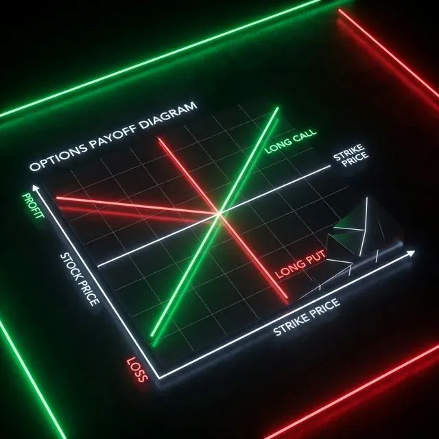Risk profiles of directional strategies (Long Call and Long Put).

There are four basic positions in options:

1. Long Call: You buy the right to buy an asset. Your profit is theoretically unlimited if the underlying asset price (S) rises. Your maximum loss is the premium (price) paid for the option.
2. Long Put: You buy the right to sell an asset. You earn when the market falls. Ideal for hedging a portfolio.
3. Short Call: You sell the right to buy. You receive the premium immediately but take on unlimited risk if the asset price "goes to the moon" (remember the GameStop short squeeze).
4. Short Put: You sell the right to sell. You receive the premium and commit to buying the asset if it falls. Often used by Warren Buffett to buy stocks at a discount.

The Breakeven point is calculated as Strike Price (X) ± Option Premium.

The Mysterious Equation: Anatomy of the Black-Scholes PDE

The formula you often see on blackboards in Wall Street movies is a partial differential equation (PDE):

Mathematical structure of the Black-Scholes model and the pricing formulas for Call and Put.

$\frac{\partial V}{\partial t} + \frac{1}{2} \sigma^2 S^2 \frac{\partial^2 V}{\partial S^2} + rS \frac{\partial V}{\partial S} - rV = 0$

Let's break it down (we promise it's not as scary as it looks):

• $V$: Option price (the value we are trying to find).
• $t$: Time. $\frac{\partial V}{\partial t}$ shows how the time value of the option decays (Theta).
• $S$: Underlying asset price (Stock/Spot).
• $\sigma$ (Sigma): Volatility of the underlying asset. The higher it is, the more expensive the option.
• $r$: Risk-free interest rate.

The equation essentially states: the return on a hedged (risk-free) portfolio consisting of options and the underlying asset must be equal to the return on a risk-free bank deposit ($rV$). This is called the no-arbitrage principle.

Practical Application: Calculating Value in Python

The analytical solution of this equation gives us the famous Black-Scholes formulas for Call and Put prices:

$C = S_0 N(d_1) - X e^{-rT} N(d_2)$ $P = X e^{-rT} N(-d_2) - S_0 N(-d_1)$

Where: $d_1 = \frac{\ln(S_0/X) + (r + \sigma^2/2)T}{\sigma \sqrt{T}}$ $d_2 = d_1 - \sigma \sqrt{T}$

Let's write this in Python. Code that turns complex math into a ready price:

import numpy as np
from scipy.stats import norm
import math

def black_scholes(S, X, T, r, sigma, option_type="call"):
    """
    Calculate option price using the Black-Scholes model.
    
    S: Current underlying asset price
    X: Strike price
    T: Time to expiration (in years)
    r: Risk-free interest rate
    sigma: Volatility of the underlying asset
    option_type: "call" or "put"
    """
    
    if T <= 0:
        if option_type == "call":
            return max(0.0, S - X)
        else:
            return max(0.0, X - S)
            
    d1 = (math.log(S / X) + (r + 0.5 * sigma**2) * T) / (sigma * math.sqrt(T))
    d2 = d1 - sigma * math.sqrt(T)
    
    if option_type == "call":
        price = S * norm.cdf(d1) - X * math.exp(-r * T) * norm.cdf(d2)
    elif option_type == "put":
        price = X * math.exp(-r * T) * norm.cdf(-d2) - S * norm.cdf(-d1)
    else:
        raise ValueError("option_type must be 'call' or 'put'")
        
    return price

current_price = 100.0   # Bitcoin at $100k (why not?)
strike_price = 100.0    # At-the-money (ATM) strike
time_to_expiry = 30/365 # 30 days to expiration
risk_free_rate = 0.05   # 5% annual rate
volatility = 0.50       # 50% volatility (typical for crypto)

call_price = black_scholes(current_price, strike_price, time_to_expiry, risk_free_rate, volatility, "call")
put_price = black_scholes(current_price, strike_price, time_to_expiry, risk_free_rate, volatility, "put")

print(f"Theoretical Call price: ${call_price:.2f}")
print(f"Theoretical Put price: ${put_price:.2f}")

Option Lords: Meet "The Greeks"

The Black-Scholes model gave us not only a price but also risk management tools known as "The Greeks". These are derivatives (gradients) of the option price with respect to various parameters:

1. Delta ($\Delta$): How much the option price changes if the underlying asset price changes by $1. (First derivative with respect to S). Delta is your directional risk.
2. Gamma ($\Gamma$): How much Delta changes if the asset price changes by $1. (Second derivative with respect to S, that very$\frac{\partial^2 V}{\partial S^2}$ from the equation). Gamma is the risk of your Delta.
3. Theta ($\Theta$): How much the option value decays per day. (Change with respect to time $t$). The enemy of the option buyer and the friend of the seller.
4. Vega ($\mathcal{V}$): How much the price changes with a 1% jump in volatility. (Spoiler: Vega is not actually a Greek letter, but it became tradition).
5. Rho ($\rho$): Sensitivity to interest rate changes. Rarely concerns crypto traders as crypto moves too fast.

Algorithmic market makers (e.g., on exchanges like Deribit or option DEXs) constantly trade the underlying asset to keep their position "Delta-neutral" ($\Delta = 0$). They earn on the spread and the divergence between Implied and Historical volatility.

Harsh Reality: Model Limitations

Black-Scholes is a brilliant formula, but it has fatal flaws in the real world, especially in crypto:

1. Constant Volatility: The formula assumes volatility is the same for all strikes. In reality, there is a "Volatility Smile" — out-of-the-money options cost more than the model predicts because traders overpay for protection against "black swans".
2. Lognormal Distribution: The model assumes prices are lognormally distributed and extreme moves are impossible. In crypto, extreme moves (Fat tails) are a regular Tuesday.
3. Continuous Trading: The formula assumes you can hedge continuously without fees. Real-world fees and slippage will quickly eat your profits.

Conclusion

The Black-Scholes formula is the Rosetta Stone of quantitative finance. Even knowing its shortcomings, the entire financial world still quotes options in units of Black-Scholes volatility.

Understanding this formula and its "Greeks" is a step from a regular trader to a quantitative researcher. Next time you decide to buy an option, remember: you are not just trading the price direction, you are trading volatility and time.

Further Reading

• Black-Scholes Model on Wikipedia
• Options: Complete Guide on Investopedia
• Derivatives and Risk Management

Code Repository

• GitHub Repository: suenot/options-pricing — full source code for the calculator and examples from the article.

Happy hedging! 📈