Assine nossa newsletter para insights exclusivos sobre trading com IA, análises de mercado e atualizações da plataforma.
Minute candles are the standard granularity for backtests. But within a single minute candle, price can move differently: sometimes by 0.01%, other times by 2%. When both stop-loss and take-profit fall within the [low, high] range of a single minute candle, the backtest doesn't know which triggered first. This is the fill ambiguity problem.
The naive solution is to switch to second-level data for the entire backtest. But over two years, that's ~63 million second bars instead of ~1 million minute bars. Storage increases 60x, speed drops proportionally.
Adaptive drill-down solves this problem: use fine granularity only where it's actually needed.
The Problem: Fill Ambiguity on Large Candles
Consider a specific situation. The strategy opened a long at 3000 USDT. Stop-loss: 2970 (-1%). Take-profit: 3060 (+2%).
The minute candle at 14:37:
Open: 3010
High: 3065
Low: 2965
Close: 3050
Both SL (2970) and TP (3060) fall within the range [2965, 3065]. Which triggered first?
Possible outcomes:
Price went down first -> SL triggered -> loss of -1%
Price went up first -> TP triggered -> profit of +2%
The difference in a single trade: 3 percentage points. With 10x leverage — 30%. For a backtest with hundreds of trades, incorrect fill ambiguity resolution systematically distorts results.
How Frameworks Handle This by Default
Most backtest engines use one of two heuristics:
Optimistic: TP triggers first -> inflated results
Pessimistic: SL triggers first -> deflated results
Both approaches are guesswork. Real data is available at second or even millisecond level, and there's no reason to guess when you can look.
Drill-Down: Three-Level Strategy
The drill-down idea: start at the minute level and "drill down" to a lower level only when there's ambiguity.
Level 1: 1m (minute candles)
  -> If SL or TP is unambiguously outside the [low, high] range — resolve on the spot
  -> If both are within the range — drill down

Level 2: 1s (second candles)
  -> Load 60 second bars for this minute
  -> Walk through second by second: which triggered first?
  -> If a second bar is also ambiguous — drill down

Level 3: 100ms (millisecond candles)
  -> Load up to 10 bars of 100ms for this second
  -> Resolve the fill at order book level
When Drill-Down Is Not Needed
In 95% of cases, drill-down is not required. Typical scenarios:
Unambiguous SL: candle high doesn't reach TP, low breaks through SL -> SL triggered, no drill-down needed.
Unambiguous TP: low doesn't reach SL, high breaks through TP -> TP triggered, no drill-down needed.
Neither triggered: both levels are outside the range -> position remains open.
Gap detection: the open of the next candle jumps through SL or TP -> execution at open price, no drill-down.
Drill-down is needed only for ~5% of bars — when both levels fall within the range of a single candle.
classAdaptiveFillSimulator:
"""
Three-level drill-down for determining fill order.
"""def__init__(self, data_loader):
self.loader = data_loader
self.cache_1s = {} # Cache of second data by monthdefcheck_fill(self, timestamp, candle_1m, sl_price, tp_price, side):
"""
Checks whether SL or TP triggered on the given minute candle.
Returns: ('sl', fill_price) | ('tp', fill_price) | None
"""
low, high = candle_1m['low'], candle_1m['high']
open_price = candle_1m['open']
if side == 'long':
if open_price <= sl_price:
return ('sl', open_price)
if open_price >= tp_price:
return ('tp', open_price)
else:
if open_price >= sl_price:
return ('sl', open_price)
if open_price <= tp_price:
return ('tp', open_price)
sl_hit = self._level_hit(sl_price, low, high, side, 'sl')
tp_hit = self._level_hit(tp_price, low, high, side, 'tp')
if sl_hit andnot tp_hit:
return ('sl', sl_price)
if tp_hit andnot sl_hit:
return ('tp', tp_price)
ifnot sl_hit andnot tp_hit:
returnNonereturnself._drill_down_1s(timestamp, sl_price, tp_price, side)
def_drill_down_1s(self, minute_ts, sl_price, tp_price, side):
"""Level 2: second-by-second pass."""
bars_1s = self.loader.load_1s_for_minute(minute_ts)
if bars_1s isNoneorlen(bars_1s) == 0:
returnself._pessimistic_fill(side, sl_price, tp_price)
for bar in bars_1s:
sl_hit = self._level_hit(sl_price, bar['low'], bar['high'], side, 'sl')
tp_hit = self._level_hit(tp_price, bar['low'], bar['high'], side, 'tp')
if sl_hit andnot tp_hit:
return ('sl', sl_price)
if tp_hit andnot sl_hit:
return ('tp', tp_price)
if sl_hit and tp_hit:
result = self._drill_down_100ms(bar['timestamp'], sl_price, tp_price, side)
if result:
return result
returnself._pessimistic_fill(side, sl_price, tp_price)
def_pessimistic_fill(self, side, sl_price, tp_price):
"""Pessimistic assumption: SL for longs, TP for shorts."""if side == 'long':
return ('sl', sl_price)
else:
return ('sl', sl_price)
Performance
Mode
Time per fill check
When used
1m (no drill-down)
~0ms
~95% of cases
1s drill-down
~5ms (first access to month)
~5% of cases
100ms drill-down
~1ms
<0.5% of cases
Over a 2-year backtest with ~400 trades, drill-down is invoked for approximately 20 candles. Total overhead — less than 1 second for the entire backtest.
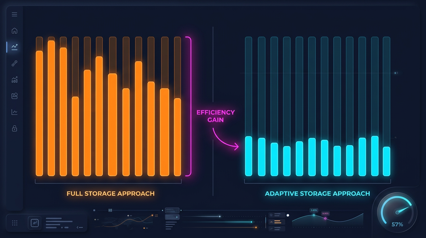
Adaptive Data Storage
Drill-down requires second and millisecond data. But storing everything at maximum granularity is impractical:
Granularity
Bars over 2 years
Parquet size
1m
~1.05M
~15 MB
1s
~63M
~550 MB/month
100ms
~630M
~5 GB/month
A complete 1s archive over 2 years is about 13 GB. 100ms — over 100 GB. Storing everything is possible but wasteful, considering that drill-down uses less than 1% of this data.
Hot-Second Detection
The key observation: seconds in which price moves significantly represent a small fraction. If price changed by less than 0.1% within a second — there's no point storing the 100ms breakdown for that second.
Hot-second detection: when downloading and processing data, we analyze each second and generate 100ms candles only for "hot" seconds — those where price movement exceeded the threshold.
defprocess_trades_adaptive(
trades: pd.DataFrame,
min_price_change_pct: float = 1.0,
) -> tuple[pd.DataFrame, pd.DataFrame]:
"""
Processes raw trades into an adaptive structure:
- 1s candles for all seconds
- 100ms candles only for "hot" seconds
Args:
trades: DataFrame with columns [timestamp, price, quantity]
min_price_change_pct: threshold for drill-down to 100ms
Returns:
(df_1s, df_100ms_hot) — second candles and 100ms for hot seconds
"""
trades['second'] = trades['timestamp'].dt.floor('1s')
df_1s = trades.groupby('second').agg(
open=('price', 'first'),
high=('price', 'max'),
low=('price', 'min'),
close=('price', 'last'),
volume=('quantity', 'sum'),
)
df_1s['price_change_pct'] = (df_1s['high'] - df_1s['low']) / df_1s['open'] * 100
hot_seconds = df_1s[df_1s['price_change_pct'] >= min_price_change_pct].index
hot_trades = trades[trades['second'].isin(hot_seconds)]
hot_trades['bucket_100ms'] = hot_trades['timestamp'].dt.floor('100ms')
df_100ms = hot_trades.groupby('bucket_100ms').agg(
open=('price', 'first'),
high=('price', 'max'),
low=('price', 'min'),
close=('price', 'last'),
volume=('quantity', 'sum'),
)
return df_1s, df_100ms
Storage Savings
For example — ETHUSDT over a typical month:
Approach
Size
Granularity
1m only
~1 MB
1 minute
All 1s
~550 MB
1 second
All 100ms
~5 GB
100 ms
Adaptive
~600 MB
1s + 100ms only for hot seconds
With a threshold of min_price_change_pct = 1.0%, hot seconds account for less than 1% of all seconds. 100ms data for them adds ~50 MB to the 550 MB of second data — a negligible overhead.
If second data is also stored adaptively (only when movement within a minute exceeds 0.1%), the volume can be reduced by another 3-5x.
DELTA_BINARY_PACKED for timestamps: consecutive timestamps differ by a fixed value (60 for 1m, 1 for 1s). Delta encoding compresses them to nearly zero.
BYTE_STREAM_SPLIT for float: splits float32 bytes into streams (all first bytes together, all second bytes together, etc.). For smoothly changing prices, this achieves 2-3x better compression than standard encoding.
ZSTD level 9: good compression with acceptable decompression speed.
float32 instead of float64: sufficient for prices and volumes, saves 50% memory.
Lazy Loading with Caching
Drill-down requests second data for a specific minute. Loading a parquet file for each request is slow. The solution — lazy loading with an LRU cache by month.
from functools import lru_cache
import pyarrow.parquet as pq
import pandas as pd
classAdaptiveDataLoader:
"""
Lazy loader with cache: loads second data by month,
keeps the last N months in memory.
"""def__init__(self, symbol: str, data_dir: str = "data", cache_months: int = 2):
self.symbol = symbol
self.data_dir = data_dir
self.cache_months = cache_months
self._cache_1s: dict[str, pd.DataFrame] = {}
defload_1s_for_minute(self, minute_ts: pd.Timestamp) -> pd.DataFrame | None:
"""Load 1s data for a specific minute."""
month_key = minute_ts.strftime("%Y-%m")
if month_key notinself._cache_1s:
self._load_month_1s(month_key)
if month_key notinself._cache_1s:
returnNone
df = self._cache_1s[month_key]
minute_start = minute_ts.floor('1min')
minute_end = minute_start + pd.Timedelta(minutes=1)
return df[(df.index >= minute_start) & (df.index < minute_end)]
defload_100ms_for_second(self, second_ts: pd.Timestamp) -> pd.DataFrame | None:
"""Load 100ms data for a hot second."""
month_key = second_ts.strftime("%Y-%m")
path = f"{self.data_dir}/{self.symbol}/klines_100ms_hot/{month_key}.parquet"try:
df = pd.read_parquet(path)
second_start = second_ts.floor('1s')
second_end = second_start + pd.Timedelta(seconds=1)
return df[(df.index >= second_start) & (df.index < second_end)]
except FileNotFoundError:
returnNonedef_load_month_1s(self, month_key: str):
"""Load a month of 1s data, evict old data from cache."""
path = f"{self.data_dir}/{self.symbol}/klines_1s/{month_key}.parquet"try:
df = pd.read_parquet(path)
df.index = pd.to_datetime(df['timestamp'], unit='s')
iflen(self._cache_1s) >= self.cache_months:
oldest = min(self._cache_1s.keys())
delself._cache_1s[oldest]
self._cache_1s[month_key] = df
except FileNotFoundError:
pass
Applying Drill-Down to Backtesting
Integration into the backtest loop:
defbacktest_with_adaptive_fill(
states: pd.DataFrame,
strategy_params: dict,
data_loader: AdaptiveDataLoader,
) -> list:
"""
Backtest with adaptive drill-down for fill simulation.
"""
fill_sim = AdaptiveFillSimulator(data_loader)
trades = []
position = Nonefor i inrange(len(states)):
row = states.iloc[i]
ts = states.index[i]
candle_1m = {
'open': row['open'], 'high': row['high'],
'low': row['low'], 'close': row['close'],
'timestamp': ts,
}
if position isnotNone:
fill = fill_sim.check_fill(
ts, candle_1m,
position['sl'], position['tp'],
position['side'],
)
if fill isnotNone:
fill_type, fill_price = fill
trades.append({
'entry_time': position['entry_time'],
'exit_time': ts,
'side': position['side'],
'entry_price': position['entry_price'],
'exit_price': fill_price,
'exit_type': fill_type,
'drill_down': fill_sim.last_drill_depth, # 0, 1, or 2
})
position = Nonecontinue
signal = check_entry_signal(row, strategy_params)
if signal and position isNone:
position = {
'side': signal['side'],
'entry_price': row['close'],
'entry_time': ts,
'sl': signal['sl'],
'tp': signal['tp'],
}
return trades
Both approaches eliminate errors invisible at the daily candle level but critical for realistic backtesting.
Summary: Fill Simulation Approach Comparison
Approach
Accuracy
Speed
Storage
OHLC heuristic (optimist/pessimist)
Low
Instant
1m only
Full 1s backtest
High
Slow (x60)
~550 MB/month
Full 100ms backtest
Maximum
Very slow (x600)
~5 GB/month
Adaptive drill-down
High
~Instant
1m + 1s + 100ms hot
Drill-down provides the accuracy of a full 1s backtest at the speed of a 1m backtest. The key observation: high granularity is not needed everywhere — only at decision points.
Conclusion
Adaptive drill-down is the application of a simple principle: spend computational resources and storage proportionally to data importance.
Three granularity levels:
1m — base pass for 95% of bars
1s — drill-down during fill ambiguity
100ms — drill-down for hot seconds with extreme movement
Three storage levels:
All 1m — complete archive, ~15 MB for 2 years
All 1s — complete or adaptive archive, ~550 MB/month
Hot 100ms only — <1% of seconds, ~50 MB/month
The result: a backtest with tick simulator accuracy at minute-level speed. And storage that grows linearly, not exponentially, with increasing granularity.
@article{soloviov2026adaptivedrilldown,
  author = {Soloviov, Eugen},
  title = {Adaptive Drill-Down: Backtest with Variable Granularity from Minutes to Milliseconds},
  year = {2026},
  url = {https://marketmaker.cc/ru/blog/post/adaptive-resolution-drill-down-backtest},
  description = {How adaptive data granularity speeds up backtests and saves storage: drill-down from 1m to 1s and 100ms only where price moved significantly.}
}