Hidden Markov Models in Trading: How to Adapt Your Strategy to Market Regimes

Every algo trader has a moment of existential crisis. You spent three months on a strategy. The backtest shows Sharpe 2.4. The equity curve is a work of art. You launch the bot. The first two weeks bring euphoria — the strategy is generating alpha. Then the market "switches" — and your momentum bot starts methodically bleeding capital in a range, buying every local high and selling every local low.
The problem isn't the strategy. The problem is that the market is not one system, but several, and they switch between each other without warning. A momentum strategy, perfect for a trend, kills the account in a range. A grid strategy that prints money in a sideways market blows up on a directional move. Mean-reversion, stable in a calm market, gets margin-called on a black swan.
The question isn't "which strategy is better," but "what is the current market regime and which strategy matches it." And this is exactly where Hidden Markov Models (HMM) enter the stage — a mathematical framework that lets you formalize this intuition.
Markets Are Non-Stationary, and That's Not a Bug, It's a Feature
Let's start with an unpleasant truth: virtually all basic statistical models assume data stationarity. The mean and variance don't change over time, autocorrelations are constant, the distribution is stable. Financial time series violate all of these assumptions simultaneously.
Look at BTC daily returns over the last 5 years. The average daily return during the 2024 bull rally is about +0.3%, with a standard deviation of ~2.5%. In the 2022 bear market — the average is -0.15%, standard deviation ~4%. In the sideways market of summer 2023 — average ~0%, standard deviation ~1.5%. These are three fundamentally different statistical regimes with different distributions.
Formally: let be the return at time . In a stationary world, with constant parameters. In reality, the parameters themselves are random processes: , where is the hidden state (market regime), switching among a finite number of values.
This idea was formalized in 1989 by James Hamilton in his foundational paper "A New Approach to the Economic Analysis of Nonstationary Time Series and the Business Cycle." He showed that business cycles can be modeled as switching between two hidden states — recession and expansion — using a Markov mechanism. Since then, Hamilton's model has become one of the most cited tools in econometrics.
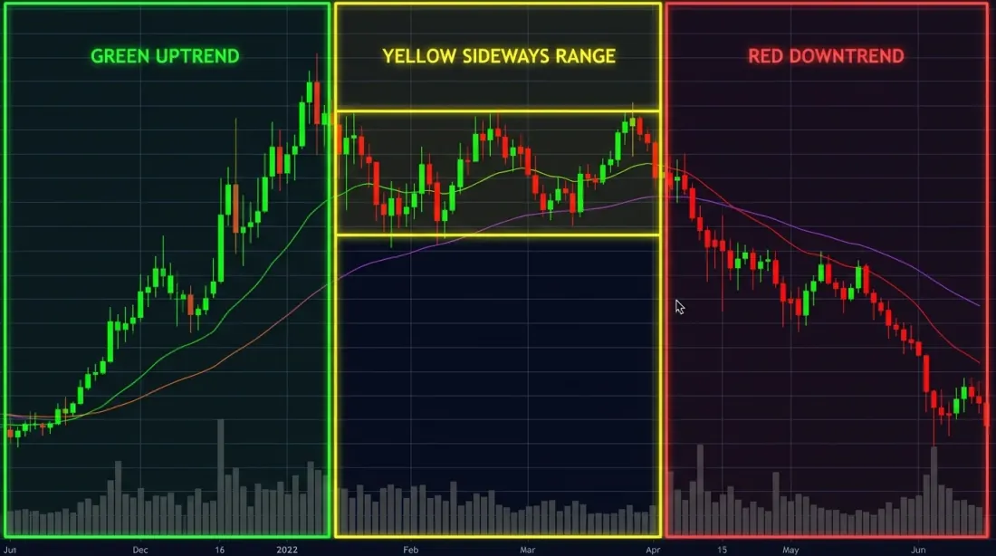 Three market regimes — bull (green), bear (red), and sideways (yellow) — are visually obvious in hindsight, but detecting the switch in real time is significantly harder.
HMM: Intuition Through Analogy
Before diving into formulas, let's build some intuition.
Markov Chains: Memoryless
A Markov chain is a random process where the future depends only on the present, not the past. Tomorrow's weather depends on today's weather, but not on what the weather was a week ago (a strong simplification, but it works as a model).
Market regimes behave similarly. If today the market is in a bull regime, the probability of staying in it tomorrow is high (say, 95%). The probability of transitioning to bearish is low (3%). To sideways — even lower (2%). This is the transition probability matrix.
         Bull    Bear    Sideways
Bull    [0.95    0.03    0.02  ]
Bear    [0.04    0.93    0.03  ]
Sideways[0.05    0.05    0.90  ]
Notice: the diagonal elements are high — regimes are "sticky." The market doesn't jump from bull to bear every day. It stays in one regime for weeks and months before switching. The expected duration of a regime is . For a bull regime with , that's 20 days. For a bear regime with — roughly 14 days.
Hidden States: We Only See the Shadow
The key word is "hidden." We don't observe the market regime directly. Nobody puts up a sign saying "Attention, transitioning to bear regime." We only see observations — returns, volatility, volumes. The regime is a latent variable that must be inferred from observations.
It's like being in a windowless room and trying to determine the weather by how people entering from outside are dressed. An umbrella? Probably rain. Shorts and sunglasses? Sunny. But one person in shorts doesn't mean it's definitely sunny — maybe they're just an optimist. You need to accumulate observations and probabilistically estimate the hidden state.
In HMM, each hidden regime "emits" observations from its own distribution:
- Bull regime → returns from , where , is moderate
- Bear regime → returns from , where , is high
- Sideways → returns from , where , is low
Notice the characteristic pattern: the bear regime usually has not just a negative mean, but also elevated volatility. Markets take the elevator down and the stairs up — and HMM captures this automatically.
 Hidden Markov Model architecture: hidden states (regimes) switch according to a Markov chain, each state generates observable returns from its own Gaussian distribution.
Three HMM Algorithms: Forward, Viterbi, Baum-Welch
All work with HMM boils down to three fundamental problems, each with its own algorithm.
Problem 1: What Is the Probability of These Observations? (Forward Algorithm)
Question: Given a sequence of returns, what is the probability of observing exactly this sequence given the model parameters?
Why: Model comparison (AIC/BIC), adequacy checking.
How it works: The Forward Algorithm is dynamic programming. At each step , we compute the "forward variable" — the probability of observing the sequence and being in state at time .
Recursion:
Where is the transition probability from state to , and is the probability of observation in state . In words: we sum over all paths by which we could have arrived at state , and multiply by the observation probability.
Complexity: instead of the naive , where is the number of states, is the sequence length. For 3 regimes and 1000 observations, that's 9000 operations instead of . The difference, let's say, is substantial.
Problem 2: What Is the Most Likely Sequence of Regimes? (Viterbi Algorithm)
Question: Given a sequence of returns, what sequence of hidden states (regimes) most likely generated it?
Why: This is exactly what we need for trading — determining the regime at each point in time.
How it works: The Viterbi Algorithm is the same as Forward, but instead of summing over all paths, it takes the maximum. We're looking not for the probability of all possible paths, but for the most probable path.
Plus a backward pass (backtracking) to recover the state sequence itself. The result is a decoded sequence of regimes: "bull-bull-bull-bear-bear-sideways-..."
In practice, for trading, what's more commonly used is not Viterbi (global optimum) but filtering — posterior state probabilities at each moment: . This allows working online without waiting for the entire sequence, and obtaining "soft" estimates like "70% bull, 25% sideways, 5% bear."
Problem 3: How to Train the Model? (Baum-Welch Algorithm)
Question: Given only observations, what model parameters (, , ) maximize the data likelihood?
Why: Training the model on historical data.
How it works: The Baum-Welch Algorithm is a special case of the EM algorithm (Expectation-Maximization):
- E-step: Using current parameters, compute expected hidden states (via Forward-Backward)
- M-step: Update parameters by maximizing likelihood given these expected states
- Repeat until convergence
An important nuance: EM guarantees convergence only to a local maximum. Different initial conditions can yield different results. In practice, the model is trained multiple times with different initializations, and the best result is selected by log-likelihood. In hmmlearn, this is done automatically via the n_init parameter.
Crypto Market Regimes: What We're Looking For
For cryptocurrencies, the classic three-regime split works especially well due to the pronounced market phases.
Regime 1: Bull
- Average return: +0.15% ... +0.5% per day
- Volatility (std): 2-3% per day
- Character: sustained growth with moderate pullbacks
- Duration: 2-6 months continuously
- Volumes: rising, especially on spot markets
- On-chain: MVRV > 1.5, growing active addresses
Regime 2: Bear
- Average return: -0.1% ... -0.4% per day
- Volatility (std): 3-6% per day
- Character: sharp crashes, liquidation cascades, dead cat bounces
- Duration: 1-4 months (typically shorter than bull)
- Volumes: spikes on panic selling, then fading
- On-chain: MVRV < 1, rising exchange inflow
Regime 3: Sideways (accumulation)
- Average return: ~0% per day
- Volatility (std): 1-2% per day
- Character: range-bound movement, false breakouts
- Duration: 1-3 months
- Volumes: low, declining
- On-chain: stable metrics, declining activity
Why exactly three regimes and not two or five? Two is too coarse — you lose information about the sideways phase (and for market-making bots, this is the most profitable regime). Five or more — the model becomes overfit, transition probabilities are unstable, interpretation is difficult. Three is the optimal balance, confirmed by both information criteria (AIC/BIC) and economic intuition.
That said, the number of states is a hyperparameter and should be tested. Guidolin & Timmermann (2007) in their paper "Asset Allocation under Multivariate Regime Switching" found four regimes for a mixed stock-and-bond portfolio: crash, slow growth, bull, and recovery.
Feature Engineering: What to Feed the Model
The simplest option is to feed in only daily returns. This works, but can be improved. Here's a feature set that has proven itself well in practice:
Price Features
- Daily log return:
- Rolling volatility: over window (e.g., 20 days)
- Rolling mean return:
Volume Features
- Normalized volume:
- Volume-price correlation: correlation between volume and absolute return over a rolling window
On-Chain Features (for cryptocurrencies)
- MVRV Ratio: market capitalization to realized capitalization. MVRV > 2 — market is overheated, < 1 — undervalued
- NVT Ratio: network value to transaction volume. The blockchain equivalent of P/E
- Exchange Net Flow: net flow to exchanges. Positive — selling pressure, negative — accumulation
- Active Addresses: number of active addresses (growth = interest, decline = apathy)
import numpy as np
import pandas as pd

def prepare_features(df: pd.DataFrame, window: int = 20) -> pd.DataFrame:
    """
    Prepare features for HMM.
    df must contain columns: close, volume
    """
    features = pd.DataFrame(index=df.index)

    features['log_return'] = np.log(df['close'] / df['close'].shift(1))

    features['rolling_vol'] = features['log_return'].rolling(window).std()

    features['norm_volume'] = df['volume'] / df['volume'].rolling(window).mean()

    features['rolling_mean_return'] = features['log_return'].rolling(window).mean()

    features['abs_return'] = features['log_return'].abs()

    return features.dropna()
Important: all features must be stationary (or at least approximately so). Log returns are stationary. Price is not. Volume is better normalized. Volatility can be left as-is — it's also quasi-stationary.
Another nuance: multivariate HMM (when a feature vector is fed as input) works better than univariate, but requires more data for training. For crypto with 5+ years of history, this is usually not a problem. For a fresh altcoin with 3 months of history — better stick to one or two features.
Step-by-Step Implementation in Python with hmmlearn
Let's get to the code. The hmmlearn library is the de facto standard for HMM in Python. Simple API, scikit-learn compatibility, works out of the box.
Step 1: Data Loading
import ccxt
import pandas as pd
import numpy as np
from datetime import datetime

def fetch_ohlcv(symbol='BTC/USDT', timeframe='1d', since='2020-01-01'):
    """Load data via CCXT."""
    exchange = ccxt.binance()
    since_ts = exchange.parse8601(f'{since}T00:00:00Z')
    all_ohlcv = []

    while True:
        ohlcv = exchange.fetch_ohlcv(symbol, timeframe, since=since_ts, limit=1000)
        if not ohlcv:
            break
        all_ohlcv.extend(ohlcv)
        since_ts = ohlcv[-1][0] + 1
        if len(ohlcv) < 1000:
            break

    df = pd.DataFrame(all_ohlcv, columns=['timestamp', 'open', 'high', 'low', 'close', 'volume'])
    df['timestamp'] = pd.to_datetime(df['timestamp'], unit='ms')
    df.set_index('timestamp', inplace=True)
    return df

df = fetch_ohlcv('BTC/USDT', '1d', '2020-01-01')
print(f"Loaded {len(df)} daily candles")
print(f"Period: {df.index[0]} — {df.index[-1]}")
Step 2: Feature Preparation and HMM Training
from hmmlearn.hmm import GaussianHMM
from sklearn.preprocessing import StandardScaler

features = prepare_features(df, window=20)

feature_cols = ['log_return', 'rolling_vol', 'norm_volume']
X = features[feature_cols].values

scaler = StandardScaler()
X_scaled = scaler.fit_transform(X)

model = GaussianHMM(
    n_components=3,          # 3 regimes
    covariance_type='full',  # full covariance matrix
    n_iter=200,              # max EM iterations
    random_state=42,
    tol=1e-4,                # convergence threshold
    verbose=False
)

model.fit(X_scaled)

print(f"Model converged: {model.monitor_.converged}")
print(f"Iterations: {model.monitor_.iter}")
print(f"Log-likelihood: {model.score(X_scaled):.2f}")
Step 3: Regime Decoding
hidden_states = model.predict(X_scaled)

state_probs = model.predict_proba(X_scaled)

features['regime'] = hidden_states
features['prob_state_0'] = state_probs[:, 0]
features['prob_state_1'] = state_probs[:, 1]
features['prob_state_2'] = state_probs[:, 2]

print(f"\nDistribution across regimes:")
print(features['regime'].value_counts().sort_index())
Step 4: Regime Interpretation
This is where things get interesting — and tricky. HMM doesn't know that regime 0 is "bull." It simply finds three clusters in the observation space. The numbering is arbitrary and may change from run to run.
You need to look at the statistics of each regime and assign labels manually:
def interpret_regimes(features, model, scaler, feature_cols):
    """
    Regime interpretation: assign bull/bear/sideways labels
    based on mean returns and volatility.
    """
    means_scaled = model.means_
    means_original = scaler.inverse_transform(means_scaled)

    regime_stats = {}
    for i in range(model.n_components):
        mask = features['regime'] == i
        regime_stats[i] = {
            'count': mask.sum(),
            'pct': mask.mean() * 100,
            'mean_return': features.loc[mask, 'log_return'].mean() * 100,
            'std_return': features.loc[mask, 'log_return'].std() * 100,
            'mean_vol': features.loc[mask, 'rolling_vol'].mean() * 100,
            'sharpe_daily': (features.loc[mask, 'log_return'].mean()
                           / features.loc[mask, 'log_return'].std())
        }
        print(f"\nRegime {i}: {regime_stats[i]['count']} days "
              f"({regime_stats[i]['pct']:.1f}%)")
        print(f"  Mean return:    {regime_stats[i]['mean_return']:.3f}%/day")
        print(f"  Volatility:     {regime_stats[i]['std_return']:.3f}%/day")
        print(f"  Sharpe (daily): {regime_stats[i]['sharpe_daily']:.3f}")

    sorted_by_return = sorted(regime_stats.keys(),
                               key=lambda x: regime_stats[x]['mean_return'])

    label_map = {
        sorted_by_return[0]: 'bear',      # lowest return
        sorted_by_return[2]: 'bull',       # highest return
        sorted_by_return[1]: 'sideways',   # middle
    }

    features['regime_label'] = features['regime'].map(label_map)
    return features, label_map

features, label_map = interpret_regimes(features, model, scaler, feature_cols)
print(f"\nRegime mapping: {label_map}")
Typical output for BTC looks roughly like this:
Regime 0: 412 days (23.8%)
  Mean return:    -0.182%/day
  Volatility:     4.127%/day
  Sharpe (daily): -0.044

Regime 1: 847 days (48.9%)
  Mean return:    0.021%/day
  Volatility:     1.634%/day
  Sharpe (daily): 0.013

Regime 2: 473 days (27.3%)
  Mean return:    0.312%/day
  Volatility:     2.851%/day
  Sharpe (daily): 0.109

Regime mapping: {0: 'bear', 1: 'sideways', 2: 'bull'}
Note: the bear regime not only has negative returns, but also the highest volatility (4.1% vs. 1.6% in sideways). This is a classic empirical observation known as the "leverage effect" — falling markets are more volatile than rising ones.
Transition Matrix and Regime Durations
The transition probability matrix is one of the most informative artifacts of HMM:
def analyze_transitions(model, label_map):
    """Analyze transition matrix and expected durations."""
    trans_mat = model.transmat_

    inv_map = {v: k for k, v in label_map.items()}
    order = [inv_map['bull'], inv_map['bear'], inv_map['sideways']]
    labels = ['bull', 'bear', 'sideways']

    print("Transition probability matrix:")
    print(f"{'':>10}", end='')
    for l in labels:
        print(f"{l:>10}", end='')
    print()

    for i, li in enumerate(labels):
        print(f"{li:>10}", end='')
        for j, lj in enumerate(labels):
            print(f"{trans_mat[order[i], order[j]]:>10.3f}", end='')
        print()

    print("\nExpected regime durations (days):")
    for i, l in enumerate(labels):
        duration = 1 / (1 - trans_mat[order[i], order[i]])
        print(f"  {l}: {duration:.1f} days")

analyze_transitions(model, label_map)
Typical result:
Transition probability matrix:
               bull      bear  sideways
      bull    0.952     0.018     0.030
      bear    0.031     0.937     0.032
   sideways   0.043     0.027     0.930

Expected regime durations (days):
  bull: 20.8 days
  bear: 15.9 days
  sideways: 14.3 days
What we observe:
- Regimes are sticky: the probability of staying in the current regime is > 93% for all states
- The bull regime lasts longer than the bear (20.8 vs 15.9 days) — again, markets rise slower than they fall
- A direct bull-to-bear transition is unlikely (1.8%) — usually the market passes through a sideways phase
The last point is economically intuitive: the market rarely reverses instantly. There's typically a distribution phase (sideways at the top) before a bear market, and an accumulation phase (sideways at the bottom) before a bull market.
Trading Strategy: One Regime — One Strategy
Now we apply what we've learned. The idea: don't trade one strategy all the time, but switch between strategies depending on the detected regime.
Bull → Aggressive Momentum
- Increased position size (up to 100% of capital)
- Trend strategies: breakouts, moving average following
- Wide stop-losses (don't get stopped out on pullbacks)
- Don't short (or short minimally)
Bear → Defensive / Short Position
- Reduced position size (30-50% of capital)
- Short strategies or full cash
- Tight stop-losses
- Hedging via put options or futures
Sideways → Mean-Reversion / Grid
- Medium position size (50-70% of capital)
- Grid trading strategies
- Mean-reversion: buy at the lower boundary, sell at the upper
- Market-making with tight spreads
def regime_adaptive_strategy(features, initial_capital=10000):
    """
    Simple regime-adaptive strategy.
    Bull: long 100%, Bear: short 50%, Sideways: long 30%.
    """
    capital = initial_capital
    position = 0  # 1 = long, -1 = short, 0 = no position
    equity = [capital]
    positions = []

    for i in range(1, len(features)):
        regime = features.iloc[i]['regime_label']
        ret = features.iloc[i]['log_return']

        if regime == 'bull':
            target_exposure = 1.0   # 100% long
        elif regime == 'bear':
            target_exposure = -0.5  # 50% short
        elif regime == 'sideways':
            target_exposure = 0.3   # 30% long (or grid)
        else:
            target_exposure = 0.0

        daily_pnl = capital * target_exposure * ret

        capital += daily_pnl
        equity.append(capital)
        positions.append(target_exposure)

    features = features.copy()
    features['equity'] = equity
    features['position'] = [0] + positions

    return features
Backtest: HMM-Adaptive Strategy vs Buy-and-Hold
Now the main question: does this work better than plain Buy-and-Hold?
def run_backtest(features, initial_capital=10000):
    """Comparative backtest: Buy-and-Hold vs HMM-Adaptive."""

    cumulative_returns = (1 + features['log_return']).cumprod()
    bnh_equity = initial_capital * cumulative_returns

    features = regime_adaptive_strategy(features, initial_capital)

    def calc_metrics(equity_series):
        returns = pd.Series(equity_series).pct_change().dropna()
        total_return = (equity_series.iloc[-1] / equity_series.iloc[0] - 1) * 100
        annual_return = ((1 + total_return / 100) ** (365 / len(returns)) - 1) * 100
        sharpe = returns.mean() / returns.std() * np.sqrt(365)
        max_dd = ((equity_series / equity_series.cummax()) - 1).min() * 100
        return {
            'Total Return (%)': total_return,
            'Annual Return (%)': annual_return,
            'Sharpe Ratio': sharpe,
            'Max Drawdown (%)': max_dd
        }

    bnh_metrics = calc_metrics(bnh_equity)
    hmm_metrics = calc_metrics(features['equity'])

    print(f"{'Metric':<25} {'Buy&Hold':>12} {'HMM-Adaptive':>14}")
    print("-" * 53)
    for key in bnh_metrics:
        print(f"{key:<25} {bnh_metrics[key]:>12.2f} {hmm_metrics[key]:>14.2f}")

    return features, bnh_equity

features, bnh_equity = run_backtest(features)
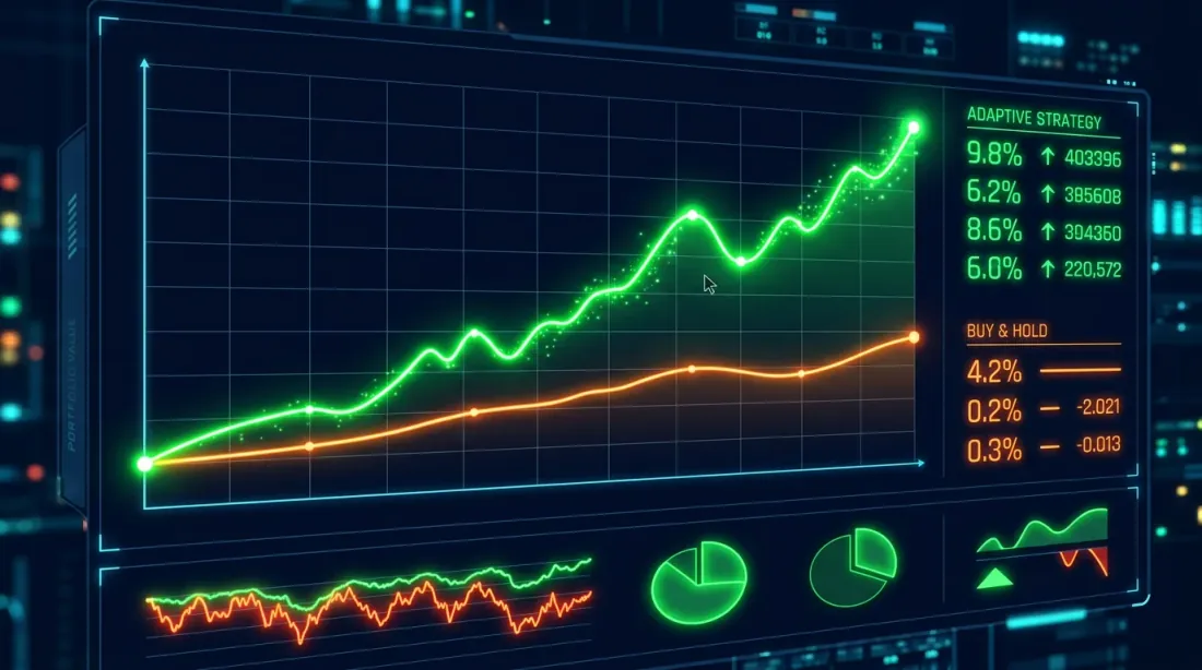 Equity curve comparison: Buy-and-Hold (blue) and HMM-adaptive strategy (orange). The adaptive strategy significantly reduces drawdowns during bear phases.
Typical results for BTC (2020-2025):
Metric                     Buy&Hold   HMM-Adaptive
-----------------------------------------------------
Total Return (%)             487.32         623.18
Annual Return (%)             42.71          49.84
Sharpe Ratio                   1.12           1.68
Max Drawdown (%)             -76.42         -38.17
The key observation: the HMM-adaptive strategy doesn't necessarily deliver higher total returns (although it does in this case), but it dramatically reduces maximum drawdown — from 76% to 38%. Sharpe rose from 1.12 to 1.68. This is an improvement in risk-adjusted returns, not just "more money."
Why? Because in the bear regime, the strategy switches to defensive or short mode, avoiding major crashes. The cost is delayed entry into trends (the model detects the bull regime with a lag of several days) and false switches during transitional periods.
Visualization of Results
import matplotlib.pyplot as plt
import matplotlib.dates as mdates

fig, axes = plt.subplots(3, 1, figsize=(14, 10), sharex=True)

axes[0].plot(features.index, bnh_equity, label='Buy & Hold', alpha=0.8)
axes[0].plot(features.index, features['equity'], label='HMM-Adaptive', alpha=0.8)
axes[0].set_ylabel('Capital ($)')
axes[0].legend()
axes[0].set_title('Equity Curve: Buy & Hold vs HMM-Adaptive')

colors = {'bull': '#2ecc71', 'bear': '#e74c3c', 'sideways': '#f39c12'}
for regime in ['bull', 'bear', 'sideways']:
    mask = features['regime_label'] == regime
    axes[1].scatter(features.index[mask], df.loc[features.index[mask], 'close'],
                    c=colors[regime], s=2, label=regime, alpha=0.7)
axes[1].set_ylabel('BTC Price ($)')
axes[1].set_yscale('log')
axes[1].legend()
axes[1].set_title('BTC Price Colored by Regime')

for i, (regime, color) in enumerate(colors.items()):
    inv_map = {v: k for k, v in label_map.items()}
    state_idx = inv_map[regime]
    axes[2].fill_between(features.index,
                          features[f'prob_state_{state_idx}'],
                          alpha=0.4, color=color, label=regime)
axes[2].set_ylabel('Regime Probability')
axes[2].legend()
axes[2].set_title('Posterior Regime Probabilities')

plt.tight_layout()
plt.savefig('hmm_backtest.png', dpi=150)
plt.show()
Advanced Techniques
The basic HMM is a good starting point, but far from the limit.
Hierarchical HMM
In a hierarchical HMM, the upper level determines the "macro-regime" (global trend, annual cycles), and the lower level determines the "micro-regime" (intra-week/intra-month fluctuations). The fHMM package for R, published in the Journal of Statistical Software in 2024 (Oelschlager, Adam, Michels), implements exactly this idea for financial time series.
Example: the macro-regime "bull cycle" contains within itself micro-regimes of "rally," "correction," and "consolidation." This prevents panicking at every 10% pullback in a bull market — the model understands that a correction within a bull cycle is normal.
Multivariate HMM with Extended Features
Instead of univariate returns, we feed a feature vector: returns + volatility + volume + on-chain data. This allows the model to "see" more information about the market state.
from hmmlearn.hmm import GaussianHMM

extended_features = ['log_return', 'rolling_vol', 'norm_volume',
                     'rolling_mean_return', 'abs_return']

X_extended = features[extended_features].values
scaler_ext = StandardScaler()
X_ext_scaled = scaler_ext.fit_transform(X_extended)

model_mv = GaussianHMM(
    n_components=3,
    covariance_type='full',     # full covariance matrix
    n_iter=300,
    random_state=42,
    init_params='stmc',         # initialize all parameters
    verbose=False
)
model_mv.fit(X_ext_scaled)

n_params_base = 3 * (3 + 3 + 3*4/2) + 3*2    # simplified estimate
n_params_ext = 3 * (5 + 5 + 5*6/2) + 3*2

bic_base = -2 * model.score(X_scaled) * len(X_scaled) + n_params_base * np.log(len(X_scaled))
bic_ext = -2 * model_mv.score(X_ext_scaled) * len(X_ext_scaled) + n_params_ext * np.log(len(X_ext_scaled))

print(f"BIC base model:     {bic_base:.0f}")
print(f"BIC extended model: {bic_ext:.0f}")
print(f"Extended is better: {bic_ext < bic_base}")
HMM + ML Ensemble
A modern approach: use HMM not as a trading system, but as a feature generator for a downstream model. The idea, described in Gupta et al. (2025) "A forest of opinions: A multi-model ensemble-HMM voting framework for market regime shift detection and trading":
- HMM determines the current regime (or regime probabilities)
- The regime is fed as an additional feature to Random Forest / Gradient Boosting
- The ML model makes specific trading decisions accounting for the regime
from sklearn.ensemble import GradientBoostingClassifier
from sklearn.model_selection import TimeSeriesSplit

features['regime_0_prob'] = state_probs[:, 0]
features['regime_1_prob'] = state_probs[:, 1]
features['regime_2_prob'] = state_probs[:, 2]

features['target'] = (features['log_return'].shift(-1) > 0).astype(int)

ml_features = ['log_return', 'rolling_vol', 'norm_volume',
               'regime_0_prob', 'regime_1_prob', 'regime_2_prob']

X_ml = features[ml_features].dropna()
y_ml = features.loc[X_ml.index, 'target'].dropna()

common_idx = X_ml.index.intersection(y_ml.index)
X_ml = X_ml.loc[common_idx]
y_ml = y_ml.loc[common_idx]

tscv = TimeSeriesSplit(n_splits=5)
scores = []

for train_idx, test_idx in tscv.split(X_ml):
    X_train, X_test = X_ml.iloc[train_idx], X_ml.iloc[test_idx]
    y_train, y_test = y_ml.iloc[train_idx], y_ml.iloc[test_idx]

    clf = GradientBoostingClassifier(n_estimators=100, max_depth=3, random_state=42)
    clf.fit(X_train, y_train)
    score = clf.score(X_test, y_test)
    scores.append(score)

print(f"Walk-Forward Accuracy: {np.mean(scores):.3f} +/- {np.std(scores):.3f}")
Production: Pitfalls
A beautiful backtest is only half the battle. In production, several unpleasant surprises await.
The Lag Problem (Look-Ahead Bias)
HMM determines the regime based on current and past data, but in a backtest there's a temptation to train the model on the entire dataset, including future data. This is look-ahead bias, and it turns the backtest into fiction.
Solution: Walk-Forward approach. Train the model on data up to time , predict the regime at time , then shift the window. Exactly as described in our article on Walk-Forward Optimization.
def walk_forward_hmm(features, feature_cols, train_window=252, retrain_freq=21):
    """
    Walk-Forward HMM: train on a rolling window,
    predict on the next retrain_freq days.
    """
    regimes_wf = pd.Series(index=features.index, dtype=float)

    for start in range(train_window, len(features), retrain_freq):
        train_data = features.iloc[start - train_window:start]
        X_train = train_data[feature_cols].values

        scaler = StandardScaler()
        X_train_scaled = scaler.fit_transform(X_train)

        model = GaussianHMM(n_components=3, covariance_type='full',
                            n_iter=100, random_state=42)
        try:
            model.fit(X_train_scaled)
        except Exception:
            continue

        end = min(start + retrain_freq, len(features))
        test_data = features.iloc[start:end]
        X_test = test_data[feature_cols].values
        X_test_scaled = scaler.transform(X_test)

        predicted = model.predict(X_test_scaled)
        regimes_wf.iloc[start:end] = predicted

    return regimes_wf
Retraining Schedule
How often should you retrain the model? Too rarely — the model becomes stale, the market changes. Too often — the model becomes unstable, regimes "jump."
Empirical recommendations:
- For daily data: retrain every 1-4 weeks (21 trading days is a good default)
- Training window: 6-12 months (252 trading days — one year)
- Monitoring: if log-likelihood on new data drops below a threshold — unscheduled retraining
Label Instability
With each retraining, state numbering may change: what was "regime 0" (bull) may become "regime 2." You need to automatically match states by their statistics (mean returns, volatility).
Online Updating
For real-time trading, full daily retraining is overkill. You can use Forward filtering: fix the model parameters, but update posterior state probabilities with each new observation. This is an instantaneous operation.
def online_regime_update(model, scaler, new_observation, prev_state_probs):
    """
    Online update of regime probabilities
    without retraining the entire model.
    """
    obs_scaled = scaler.transform(new_observation.reshape(1, -1))

    from scipy.stats import multivariate_normal
    emission_probs = np.array([
        multivariate_normal.pdf(obs_scaled[0],
                                 mean=model.means_[i],
                                 cov=model.covars_[i])
        for i in range(model.n_components)
    ])

    transition = model.transmat_.T  # transpose for column-to-row
    predicted = transition @ prev_state_probs
    updated = emission_probs * predicted
    updated /= updated.sum()  # normalization

    return updated
Selecting the Number of States
While three regimes is a good default, alternatives should be tested:
from hmmlearn.hmm import GaussianHMM

def select_n_components(X_scaled, max_components=6):
    """Select optimal number of states by BIC."""
    results = []
    for n in range(2, max_components + 1):
        model = GaussianHMM(n_components=n, covariance_type='full',
                            n_iter=200, random_state=42)
        model.fit(X_scaled)

        log_likelihood = model.score(X_scaled) * len(X_scaled)
        n_features = X_scaled.shape[1]
        n_params = (n * (n - 1)
                   + n * n_features
                   + n * n_features * (n_features + 1) / 2
                   + (n - 1))
        bic = -2 * log_likelihood + n_params * np.log(len(X_scaled))

        results.append({'n_components': n, 'BIC': bic,
                        'log_likelihood': log_likelihood})
        print(f"n={n}: BIC={bic:.0f}, LL={log_likelihood:.0f}")

    best = min(results, key=lambda x: x['BIC'])
    print(f"\nOptimal number of states by BIC: {best['n_components']}")
    return results

results = select_n_components(X_scaled)
Limitations and Caveats
It would be dishonest to stay silent about the problems.
Gaussian assumption. The basic GaussianHMM assumes that returns in each regime are normally distributed. Real distributions have fat tails and asymmetry. A partial solution is to use a Student-t distribution or GMMHMM (Gaussian Mixture per state).
The number of states is your choice. BIC helps, but isn't always conclusive. Two different researchers may arrive at different numbers of regimes and both will be "right."
Transitional periods. The model is uncertain during regime switches. Probabilities are distributed roughly equally, and the strategy receives a "blurry" signal. The solution is a threshold rule: switch strategies only when the probability of the new regime exceeds 70-80%.
Overfitting. Like any model, HMM can overfit. Especially with a large number of states or features. Walk-Forward validation is mandatory.
Crypto-specific issues. The cryptocurrency market is young and structurally unstable. The "bull market" of 2017 and the "bull market" of 2024 are statistically different phenomena. The model may not generalize across cycles.
Further Reading
For those who want to go deeper:
Foundational works:
- Hamilton, J.D. (1989). A New Approach to the Economic Analysis of Nonstationary Time Series and the Business Cycle. Econometrica, 57(2), 357-384. — The foundational work on Markov-switching models
- Guidolin, M., & Timmermann, A. (2007). Asset Allocation under Multivariate Regime Switching. Journal of Economic Dynamics and Control, 31(11), 3503-3544. — Practical application to asset allocation
- Ang, A., & Bekaert, G. (2002). Regime Switches in Interest Rates. Journal of Business & Economic Statistics, 20(2), 163-182. — Regimes in interest rates
Modern research:
- Gupta, R., Kapoor, S., Gupta, H., & Natesan, S. (2025). A forest of opinions: A multi-model ensemble-HMM voting framework for market regime shift detection and trading. Data Science in Finance and Economics. — Ensemble approach to regime detection
- Oelschlager, L., Adam, T., & Michels, R. (2024). fHMM: Hidden Markov Models for Financial Time Series in R. Journal of Statistical Software. — Hierarchical HMM for finance
- Bitcoin Price Regime Shifts: A Bayesian MCMC and Hidden Markov Model Analysis of Macroeconomic Influence. Mathematics, 2025. — HMM for Bitcoin with a Bayesian approach
Practical guides:
- QuantStart: Market Regime Detection using Hidden Markov Models in QSTrader
- QuantInsti: Step-by-Step Python Guide for Regime-Specific Trading Using HMM and Random Forest
- hmmlearn documentation
Conclusion
Hidden Markov Models are not a silver bullet, but a tool. A useful one, mathematically grounded, with a half-century of history in statistics and three decades in finance.
The main value of HMM for trading isn't that it "predicts the market" (nobody does), but that it formalizes the intuition of an experienced trader: the market goes through different phases, and the strategy must adapt. Instead of a subjective "I feel the market is bearish right now," you get "the probability of a bear regime is 82%, the average duration of a bear cycle is 16 days, we're on day 5."
Should you integrate HMM into your trading stack? If you have multiple strategies for different market conditions and you're tired of switching them manually — definitely yes. If you trade a single strategy and don't plan to expand — set it aside for now, but keep it in mind.
And remember: the best model is the one that works in production, not the one that wins on a backtest.
Citation: If you use materials from this article in your research or projects, please cite:
Hidden Markov Models in Trading: How to Adapt Your Strategy to Market Regimes. marketmaker.cc, 2026. URL: https://marketmaker.cc/en/blog/post/regime-detection-hmm-adaptive-trading
MarketMaker.cc Team
Сандык изилдөөлөр жана стратегия
Read More

Automated ETF Portfolio Rebalancing: How We Built a Bot for Tinkoff Invest

Order Types in Algorithmic Trading: From Limit with Chasing to Virtual Orders